# --- Google Colab bootstrap; does nothing anywhere else ---------------------
import importlib.util, pathlib, subprocess, sys, urllib.error, urllib.request

IN_COLAB = importlib.util.find_spec("google.colab") is not None

# `main` once this is merged; the branch is the fallback so the Colab path can
# be tested BEFORE the merge, when main does not yet have these files.
_REFS = ("main", "af-day3-final-cleanup")
_RAW = "https://raw.githubusercontent.com/stefanradev93/sbi4cogsci/{ref}/tutorials/"


def _fetch(path, dest=None):
    """Download `path` (relative to `tutorials/`) to `dest`, default its basename."""
    dest = dest or path.rsplit("/", 1)[-1]
    for ref in _REFS:
        try:
            urllib.request.urlretrieve(_RAW.format(ref=ref) + path, dest)
            return ref
        except urllib.error.HTTPError:
            continue
    raise RuntimeError(f"could not fetch {path} from any of {_REFS}")


if IN_COLAB:
    # numba>=0.61 is REQUIRED, not cosmetic. pytensor resolves linker="auto" to
    # its numba backend, and numba renamed FunctionModel's first field
    # addr -> c_addr in 0.61. Colab preinstalls an older numba, and pytensor
    # declares numba only as an optional extra, so pip leaves it in place and
    # any MvNormal (SolveTriangular has no C implementation) dies with
    # KeyError: "FunctionModel does not have a field named 'c_addr'".
    # bayesflow pulls keras 3, which section 7 needs — without it the notebook
    # dies at `import bayesflow` rather than anywhere informative.
    subprocess.run([sys.executable, "-m", "pip", "install", "-q",
                    "numba>=0.61", "pymc>=6.2", "arviz>=1.2", "hssm>=0.4",
                    "bayesflow>=2.0"],
                   check=True)
    # `dot` is a system binary, not a Python package.
    subprocess.run(["apt-get", "-qq", "install", "-y", "graphviz"],
                   check=True)
    for _mod in ["sbi4cogsci_style.py"]:
        print(f"  fetched {_mod} from {_fetch(_mod)}")
    # Section 7 LOADS a trained network rather than training one. Skip this and
    # `CKPT.exists()` is False on Colab, so that cell silently drops into its
    # training branch — 150 epochs x 300 batches, roughly 25 minutes.
    pathlib.Path("checkpoints").mkdir(exist_ok=True)
    _ck = "day3_sbi_tools/checkpoints/ddm_nre.keras"
    print(f"  fetched ddm_nre.keras from "
          f"{_fetch(_ck, 'checkpoints/ddm_nre.keras')}")
print("Colab setup done.")HSSM in thirty minutes
Day 3, 09:30 — 30 minutes. Alexander Fengler.

Yesterday at 12:00 you saw bambi: write "y ~ 1 + x", and it builds the PyMC model, chooses priors, fits, and predicts at new covariates. At 14:30 you dropped a DDM likelihood into PyMC by hand and wrote v[coh_idx] to make drift depend on condition.
HSSM is what you get when you combine those two ideas. It is a formula interface — built on bambi — for models whose likelihood is a sequential-sampling model rather than a Gaussian. The extra axes of flexibility it adds over bambi are:
| bambi | HSSM | |
|---|---|---|
| likelihood | GLM families | DDM, LBA, race, collapsing-bound, … |
| what a formula acts on | parameters of the family | translates to any SSM parameter — drift, boundary, bias, non-decision time |
| where the likelihood comes from | closed form | closed form, a neural approximation, or your own function |
| extras features | — | native lapse processes, proprietary plots, “surrogate -> PyMC RV” constructors |
▶️ Running this on Google Colab
The cell below is a no-op on your own machine. On Colab it installs the stack and downloads the shared helper module, which lives one directory up in the repository and is therefore not importable there.
Expect the install to take a few minutes. If Colab asks you to restart the runtime, do it and then run the cell again — the second run is a no-op.
import sys, pathlib, warnings
sys.path.insert(0, str(pathlib.Path.cwd().parent))  # -> tutorials/

import numpy as np
import pandas as pd
import matplotlib.pyplot as plt
import arviz as az
import hssm
import sbi4cogsci_style as S

S.use()
warnings.filterwarnings("ignore")

RANDOM_SEED = sum(map(ord, "sbi4cogsci-hssm"))
rng = np.random.default_rng(RANDOM_SEED)
PARAMS = ["v", "a", "z", "t"]

print("hssm", hssm.__version__, "|", len(hssm.list_models()), "built-in models")
hssm 0.4.0 | 16 built-in models1. A dataset whose truth we know
We could load a real dataset. Instead we build one from a known model, so that every claim about recovery later is checkable rather than rhetorical.
The design is modelled on cavanagh_theta, the classic dataset shipped with HSSM: participants, a trial-level covariate, and a condition.
The generative model is
\[ v_i = \beta^v_0 + \beta^v_1\, \mathbb{1}[\text{cond}_i = \text{"hard"}], \qquad a_i = \beta^a_0 + \beta^a_1\, \text{theta}_i, \]
with \(z\) and \(t\) fixed. Difficulty acts on the drift — a harder stimulus supplies weaker evidence — and theta acts on the boundary.
That assignment is a modelling claim, not a convenience. It matches what cavanagh_theta is famous for — mediofrontal theta tracks the decision threshold, not the rate of evidence accumulation — and it makes the two manipulations visibly different: drift moves accuracy and RT together, boundary trades them off. The exercise at the end asks what happens if you swap them.
N_TRIALS = 1200
theta_cov = rng.normal(0.0, 1.0, N_TRIALS)               # trial-level covariate
cond = rng.choice(["easy", "hard"], N_TRIALS)

scaffold = hssm.simulate_data("ddm", [0.5, 1.5, 0.5, 0.3], N_TRIALS,
                              random_state=RANDOM_SEED)
scaffold["theta"] = theta_cov
scaffold["cond"] = cond

# The generating model. p_outlier=None so the synthetic data contains no
# lapses; center_predictors=False so an Intercept means "the value at 0".
gen_model = hssm.HSSM(
    data=scaffold, model="ddm",
    include=[{"name": "v", "formula": "v ~ 1 + C(cond)"},
             {"name": "a", "formula": "a ~ 1 + theta"}],
    p_outlier=None, center_predictors=False,
)

# Every free parameter must be pinned, and each value must match that
# parameter's SHAPE. Categorical contrasts are vectors even when there is only
# one of them — `v_C(cond)` has shape (1,), so it takes [-0.4], not -0.4.
#
# The two drift values are chosen to land both conditions in the 15-35% error
# band that yesterday afternoon identified as the well-conditioned regime:
# easy ends up near 14% errors, hard near 36%.
TRUE = {
    "v_Intercept": 0.6,      # drift in the "easy" condition
    "v_C(cond)": [-0.4],     # how much WEAKER the evidence is when "hard"
    "a_Intercept": 1.5,      # boundary at theta = 0
    "a_theta": 0.3,          # boundary per unit of theta
    "z": 0.5,
    "t": 0.30,
}
print("free parameters and their shapes:")
for rv, val in gen_model.pymc_model.initial_point().items():
    print(f"   {rv:24s} {val.shape}")

# `sample_do` pins every free parameter to a chosen value and draws from the
# resulting model — the do-operator you met yesterday, used generatively.
dt = gen_model.sample_do(TRUE, draws=1, random_seed=RANDOM_SEED)
sim = dt["prior_predictive"]["rt,response"].values[0, 0]     # (N_TRIALS, 2)

data = pd.DataFrame(sim, columns=["rt", "response"])
data["theta"] = theta_cov
data["cond"] = cond
data["participant_id"] = rng.integers(0, 12, N_TRIALS)       # for section 6

print(data.head().to_string(index=False))
print(f"\n{len(data)} trials | error rate {(data['response'] == -1).mean():.1%}")
Model initialized successfully.Sampling: [rt,response]free parameters and their shapes:
z_interval__ ()
t_log__ ()
v_Intercept ()
v_C(cond) (1,)
a_Intercept_interval__ ()
a_theta ()
rt response theta cond participant_id
2.453736 1.0 1.293487 hard 4
1.036704 1.0 -0.930231 hard 11
2.971241 1.0 -0.313631 easy 10
2.307350 1.0 0.472591 easy 10
9.768160 1.0 0.424181 hard 0
1200 trials | error rate 25.2%🔑 Response coding in HSSM
Two-choice models expect responses coded -1 and +1. You never have to guess this — every model declares it:
hssm.config.model_config["ddm"]["choices"] -> [-1, 1]Multi-alternative models use [0 … K-1] instead, and declare that the same way. Check the config rather than assuming.
from ssms.config import model_config
for name in ["ddm", "angle", "lba3", "race_no_bias_angle_4"]:
    print(f"  {name:22s} choices = {model_config[name]['choices']}")
ddm choices = [-1, 1]
angle choices = [-1, 1]
lba3 choices = [0, 1, 2]
race_no_bias_angle_4 choices = [0, 1, 2, 3]2. The shortest model that works
One line for the model, one for the fit.
model_flat = hssm.HSSM(data=data, model="ddm")
print(model_flat)
Model initialized successfully.
Hierarchical Sequential Sampling Model
Model: ddm
Response variable: rt,response
Likelihood: analytical
Observations: 1200
Parameters:
v:
Prior: Normal(mu: 0.0, sigma: 2.0)
Explicit bounds: (-inf, inf)
a:
Prior: HalfNormal(sigma: 2.0)
Explicit bounds: (0.0, inf)
z:
Prior: Uniform(lower: 0.0, upper: 1.0)
Explicit bounds: (0.0, 1.0)
t:
Prior: HalfNormal(sigma: 2.0)
Explicit bounds: (0.0, inf)
Lapse probability: 0.05
Lapse distribution: Uniform(lower: 0.0, upper: 20.0)print(model) resolves and shows every prior, every bound, the links, and the lapse process. Read it before sampling, every time.
The graph shows the same thing structurally:
model_flat.graph()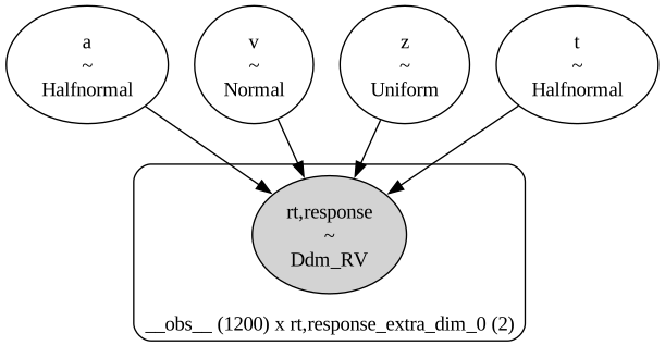
model_flat.sample(draws=500, tune=500, chains=2, cores=1,
                  random_seed=RANDOM_SEED, progressbar=False)
print(az.summary(model_flat.traces, var_names=PARAMS, kind="stats").to_string())
Using default initvals.
Initializing NUTS using adapt_diag...
Sequential sampling (2 chains in 1 job)
NUTS: [a, t, z, v]
Sampling 2 chains for 500 tune and 500 draw iterations (1_000 + 1_000 draws total) took 7 seconds.
We recommend running at least 4 chains for robust computation of convergence diagnostics
mean sd eti89_lb eti89_ub
v 0.4 0.028 0.35 0.44
a 1.5 0.024 1.4 1.5
z 0.49 0.011 0.47 0.51
t 0.23 0.02 0.2 0.263. p_outlier: the lapse process
Notice the last line of print(model): Lapse probability: 0.05. Every HSSM model carries one unless you say otherwise, and it is worth understanding rather than merely knowing about.
Real response-time data contains trials the model did not generate — button mashing, attention lapses, a sneeze. Those trials have RTs the SSM considers nearly impossible, and because the likelihood is a product over trials, one impossible trial can dominate the entire fit.
HSSM’s answer is a mixture. With lapse probability \(p\) and lapse density \(f_{\text{lapse}}\),
\[ f_{\text{eff}}(\text{rt}) \;=\; (1-p)\, f_{\text{SSM}}(\text{rt}) \;+\; p\, f_{\text{lapse}}(\text{rt}), \]
with \(f_{\text{lapse}}\) defaulting to \(\text{Uniform}(0, 20)\). The effect is a floor: no observation can ever be more surprising than \(\log(p/20)\).
import pymc as pm

probe = pd.DataFrame({"rt": [0.9, 0.31, 18.0], "response": [1.0, 1.0, -1.0]})
THETA = dict(v=2.0, a=2.5, z=0.5, t=0.3)

m_on = hssm.HSSM(data=probe, model="ddm", p_outlier=0.05, a=2.5, z=0.5, t=0.3)
m_off = hssm.HSSM(data=probe, model="ddm", p_outlier=None, a=2.5, z=0.5, t=0.3)

obs = probe[["rt", "response"]].to_numpy()
lp_off = pm.logp(m_off.model_distribution.dist(**THETA), obs).eval()
lp_on = pm.logp(m_on.model_distribution.dist(**THETA, p_outlier=0.05), obs).eval()

print(f"{'rt':>7} {'no lapse':>12} {'with lapse':>12}")
for r, off, on in zip(probe["rt"], lp_off, lp_on):
    print(f"{r:7.2f} {off:12.2f} {on:12.2f}")
print(f"\nthe floor is log(p/20) = {np.log(0.05 / 20):.3f}")
Model initialized successfully.
Model initialized successfully.
rt no lapse with lapse
0.90 -0.64 -0.69
0.31 -64.34 -5.99
18.00 -45.97 -5.99
the floor is log(p/20) = -5.991The typical trial barely moves. The impossibly fast one (rt below the non-decision time, so the SSM says it cannot happen) goes from \(-64\) to the floor, and the very slow one likewise. Draw it:
rt_grid = np.linspace(0.05, 6.0, 400)
grid_df = pd.DataFrame({"rt": rt_grid, "response": np.ones_like(rt_grid)})
m_g_off = hssm.HSSM(data=grid_df, model="ddm", p_outlier=None, a=2.5, z=0.5, t=0.3)
dens_ssm = np.exp(pm.logp(m_g_off.model_distribution.dist(**THETA),
                          grid_df[["rt", "response"]].to_numpy()).eval())

fig, axes = plt.subplots(1, 2, figsize=(11, 3.8))
for ax, logscale in zip(axes, [False, True]):
    ax.plot(rt_grid, dens_ssm, color=S.NAIVE, lw=2, label="SSM only ($p=0$)")
    for p, colour, ls in [(0.05, S.PRIMARY, "-"), (0.20, S.ALT, "--")]:
        ax.plot(rt_grid, (1 - p) * dens_ssm + p * (1 / 20),
                color=colour, ls=ls, lw=2, label=f"with lapse, $p={p}$")
    ax.set(xlabel="RT (s)", ylabel="density",
           title="effective likelihood" + (" (log scale)" if logscale else ""))
    if logscale:
        ax.set_yscale("log")
    ax.legend(fontsize=9)
fig.tight_layout()
Model initialized successfully.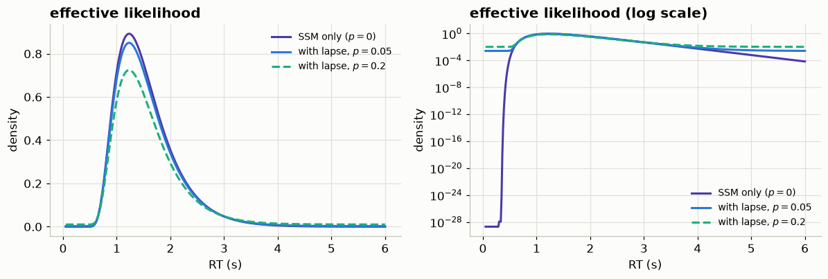
On the linear scale the mixture is indistinguishable from the SSM density — that is the point, it barely touches the trials the model explains well. On the log scale you can see what it actually does: it holds the density up off zero everywhere, so no single trial can contribute an unboundedly large negative log-likelihood.
4. Fit checks that are specific to SSMs
A trace plot tells you the sampler behaved. It says nothing about whether the model describes the data.
The quantile probability plot is the field standard: RT quantiles on the y-axis against choice proportion on the x-axis, so speed and accuracy appear together, split by condition. Ellipses summarise the posterior-predictive spread more legibly than a point cloud.
model_flat.sample_posterior_predictive(kind="response", draws=100)
ax = model_flat.plot_quantile_probability(cond="cond", predictive_style="ellipse",
                                          ellipse_confidence=0.95)
# The method returns its Axes, so the y-limits are yours to set. Do set them:
# the default view clips to the observed quantiles, which slices the tops off
# the predictive ellipses and hides exactly the misfit you are looking for.
ax.set_ylim(0, 5)
plt.gcf().set_size_inches(7.5, 4.5)
plt.gcf().suptitle("Flat model — one drift, one boundary", y=1.02)
plt.tight_layout()
dt=None, we use the traces assigned to the HSSM object as datatree.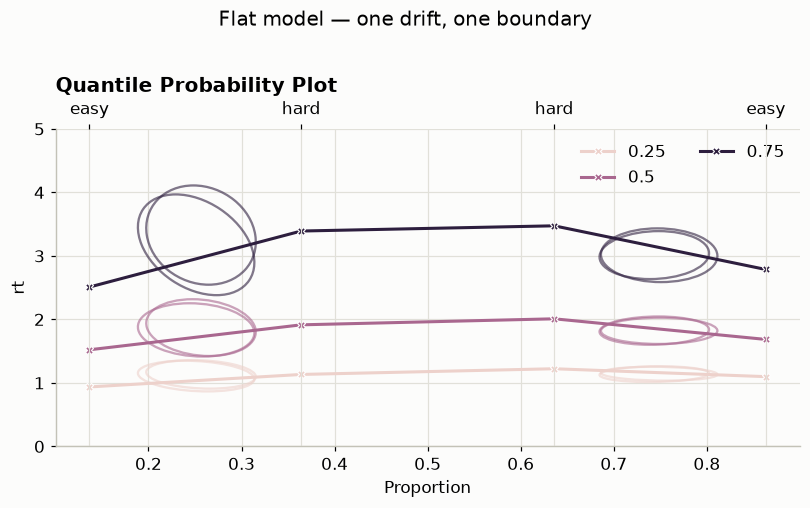
The model cartoon draws the fitted process itself: boundaries, start point, drift and non-decision time, with the observed RT histograms mirrored above and below.
Two arguments make it show uncertainty rather than a single tidy summary. plot_predictive_samples=True draws one boundary-and-drift sketch per posterior draw, so the grey fan is the posterior on the parameters; n_trajectories overlays actual simulated paths. The mean drift is not what any single trial does.
hssm.plotting.plot_model_cartoon(model_flat, n_samples=20,
                                 plot_predictive_samples=True,
                                 n_trajectories=3)
plt.gcf().set_size_inches(7.5, 4)
plt.tight_layout()
No posterior_predictive samples found. Generating posterior_predictive samples using the provided DataTree object and the original data. This will modify the provided DataTree object, or if not provided, the traces object stored inside the model.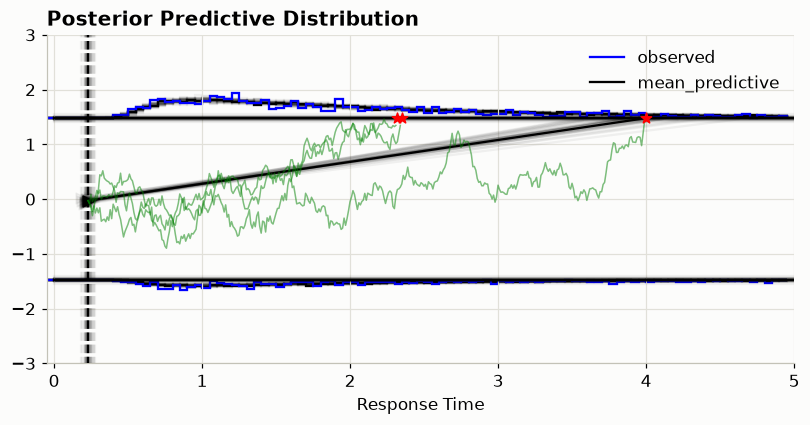
5. A more accurate model
The flat model has one drift and one boundary for every trial, but we built this dataset so that drift depends on cond and boundary tracks theta. In HSSM that is a formula per parameter — the bambi idea, applied to the inside of a cognitive model.
model_reg = hssm.HSSM(
    data=data, model="ddm",
    include=[{"name": "v", "formula": "v ~ 1 + C(cond)"},
             {"name": "a", "formula": "a ~ 1 + theta"}],
    p_outlier=0.05,
)
model_reg.graph()
Model initialized successfully.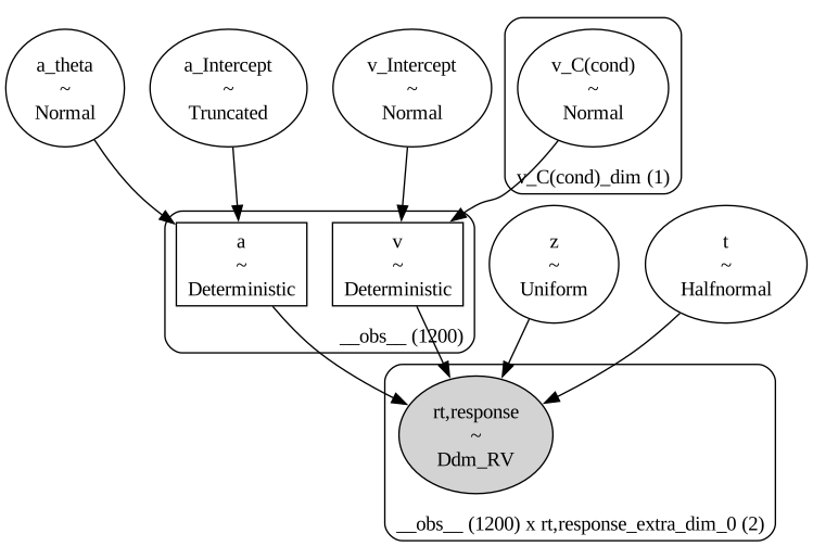
model_reg.sample(draws=500, tune=500, chains=2, cores=1,
                 random_seed=RANDOM_SEED, progressbar=False)
print(az.summary(model_reg.traces,
                 var_names=["v_Intercept", "v_C(cond)", "a_Intercept",
                            "a_theta", "z", "t"],
                 kind="stats").to_string())
print("\nTRUE:", {k: v for k, v in TRUE.items()})
Using default initvals.
Initializing NUTS using adapt_diag...
Sequential sampling (2 chains in 1 job)
NUTS: [t, z, v_Intercept, v_C(cond), a_Intercept, a_theta]
Sampling 2 chains for 500 tune and 500 draw iterations (1_000 + 1_000 draws total) took 9 seconds.
We recommend running at least 4 chains for robust computation of convergence diagnostics
mean sd eti89_lb eti89_ub
v_Intercept 0.67 0.039 0.6 0.73
v_C(cond)[hard] -0.44 0.045 -0.52 -0.37
a_Intercept 1.5 0.023 1.5 1.5
a_theta 0.27 0.017 0.24 0.29
z 0.49 0.011 0.47 0.51
t 0.3 0.015 0.27 0.32
TRUE: {'v_Intercept': 0.6, 'v_C(cond)': [-0.4], 'a_Intercept': 1.5, 'a_theta': 0.3, 'z': 0.5, 't': 0.3}model_reg.sample_posterior_predictive(kind="response", draws=100)
ax = model_reg.plot_quantile_probability(cond="cond", predictive_style="ellipse",
ellipse_confidence=0.95)
ax.set_ylim(0, 5) # same y-range as the flat model, so the two compare
plt.gcf().set_size_inches(7.5, 4.5)
plt.gcf().suptitle("Regression model — drift ~ condition, boundary ~ theta", y=1.02)
plt.tight_layout()dt=None, we use the traces assigned to the HSSM object as datatree.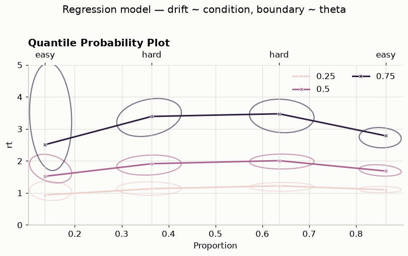
How to read a quantile probability plot
The standard fit check for sequential-sampling models, and worth learning to read properly because it shows accuracy and RT at the same time.
- Horizontal axis — the proportion of responses in that group. Each condition contributes two points: errors on the left, correct responses on the right, mirrored about 0.5.
- Vertical axis — the 25th, 50th and 75th RT percentiles, so the vertical spread is the shape of the RT distribution.
- Ellipses — the posterior predictive. The model fits where they cover the observed points.
The four x-positions read outward from the centre as: hard errors, hard correct, easy errors, easy correct. Compare it with the flat model above, which collapses both conditions onto a single pair of positions — a single drift cannot produce two accuracies.
💡 This is the key argument for HSSM
include=[{"name": "v", "formula": "v ~ 1 + C(cond)"}] replaced the v[coh_idx] indexing you wrote by hand yesterday — and it extends to random effects, multiple parameters, and link functions without you writing any of it.
Exercise
Fit a model where the mapping is swapped: drift depends on theta and boundary on cond. It has exactly the same number of parameters. Compare its quantile probability plot to the one above, and predict first — which of the two axes of the plot will it get wrong?
What to notice
swapped = hssm.HSSM(
    data=data, model="ddm",
    include=[{"name": "v", "formula": "v ~ 1 + theta"},
             {"name": "a", "formula": "a ~ 1 + C(cond)"}])
swapped.sample(draws=500, tune=500, chains=2, cores=1, progressbar=False)
swapped.sample_posterior_predictive(kind="response", draws=100)
swapped.plot_quantile_probability(cond="cond", predictive_style="ellipse")
The horizontal axis is the one that collapses. Boundary height barely moves accuracy when the start point is unbiased — raising a makes both responses slower and leaves their ratio almost untouched — so a model that puts the condition effect on a predicts the two conditions at nearly the same proportion. Its predicted ellipses stack up in two vertical columns while the observed points sit at four clearly separated positions.
It still fits far better than the flat model, and it has the right number of parameters. That is the trap: the right number of parameters is not the same as the right model, and a summary table of coefficients will not tell you — the fit check will.
This is also a design lesson, not only a modelling one. If your manipulation only ever moves the boundary, a quantile probability plot has almost no horizontal spread to check against, and you have thrown away the axis that makes the model falsifiable.
6. Hierarchical regression
Real designs have participants. HSSM takes bambi’s random-effects syntax directly, so a participant-level drift intercept is (1|participant_id).
model_hier = hssm.HSSM(
    data=data, model="ddm",
    include=[{"name": "v", "formula": "v ~ 1 + C(cond) + (1|participant_id)"},
             {"name": "a", "formula": "a ~ 1 + theta"}],
    noncentered=True,          # see Day 3, 11:00 for why this matters
    p_outlier=0.05,
    prior_settings="safe",
)
model_hier.graph()
Model initialized successfully.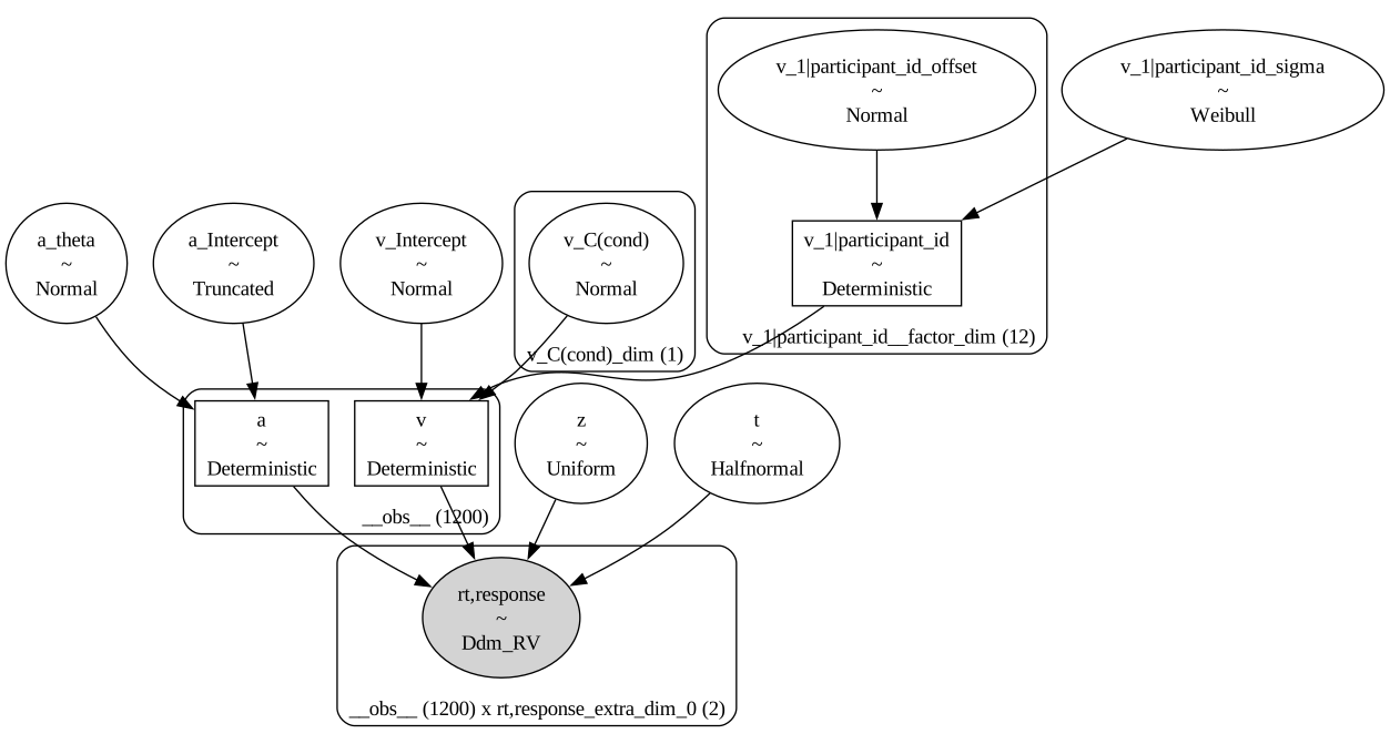
model_hier.sample(draws=500, tune=500, chains=2, cores=1,
                  random_seed=RANDOM_SEED, progressbar=False)
print(az.summary(model_hier.traces,
                 var_names=["v_Intercept", "v_C(cond)", "v_1|participant_id_sigma",
                            "a_Intercept", "a_theta"],
                 kind="stats").to_string())
Using default initvals.
Initializing NUTS using adapt_diag...
Sequential sampling (2 chains in 1 job)
NUTS: [t, z, v_Intercept, v_C(cond), v_1|participant_id_sigma, v_1|participant_id_offset, a_Intercept, a_theta]
Sampling 2 chains for 500 tune and 500 draw iterations (1_000 + 1_000 draws total) took 33 seconds.
We recommend running at least 4 chains for robust computation of convergence diagnostics
mean sd eti89_lb eti89_ub
v_Intercept 0.67 0.04 0.6 0.73
v_C(cond)[hard] -0.44 0.046 -0.52 -0.37
v_1|participant_id_sigma 0.04 0.024 0.0081 0.084
a_Intercept 1.5 0.023 1.5 1.5
a_theta 0.27 0.017 0.24 0.29v_1|participant_id_sigma is the population spread of participant drift intercepts. Our synthetic participants were assigned at random, so it should be near zero — and a hierarchical model that correctly reports “there is no participant variance here” is doing its job.
The geometry of that sigma parameter is what the 11:00 session is about.
A forest plot is the natural summary for a hierarchical fit: every coefficient on one axis, with intervals you can scan for overlap with zero.
One filter first. A fitted posterior can hold two kinds of variable: a handful of coefficients, and — depending on the model — deterministics carrying one entry per trial. Hand the second kind to plot_forest and it will dutifully draw thousands of rows. Select on the dimensions, not by listing names that go stale the moment you edit a formula:
post = model_hier.traces.posterior
n_obs = len(data)

coef_vars = [
    v for v in post.data_vars
    # keep anything with no trial-sized axis
    if not any(post[v].sizes[d] == n_obs for d in post[v].dims)
]
print(f"{len(post.data_vars)} posterior variables -> {len(coef_vars)} coefficients")
print("dropped:", sorted(set(post.data_vars) - set(coef_vars)) or "nothing (this model stores only coefficients)")
9 posterior variables -> 9 coefficients
dropped: nothing (this model stores only coefficients)az.plot_forest(model_hier.traces, var_names=coef_vars, combined=True)
fig = plt.gcf()
for ax in fig.axes: # a zero line to read "overlaps zero" off
ax.axvline(0.0, color="0.4", ls=":", lw=1)
fig.suptitle("Hierarchical fit — all coefficients", y=1.01)
fig.tight_layout()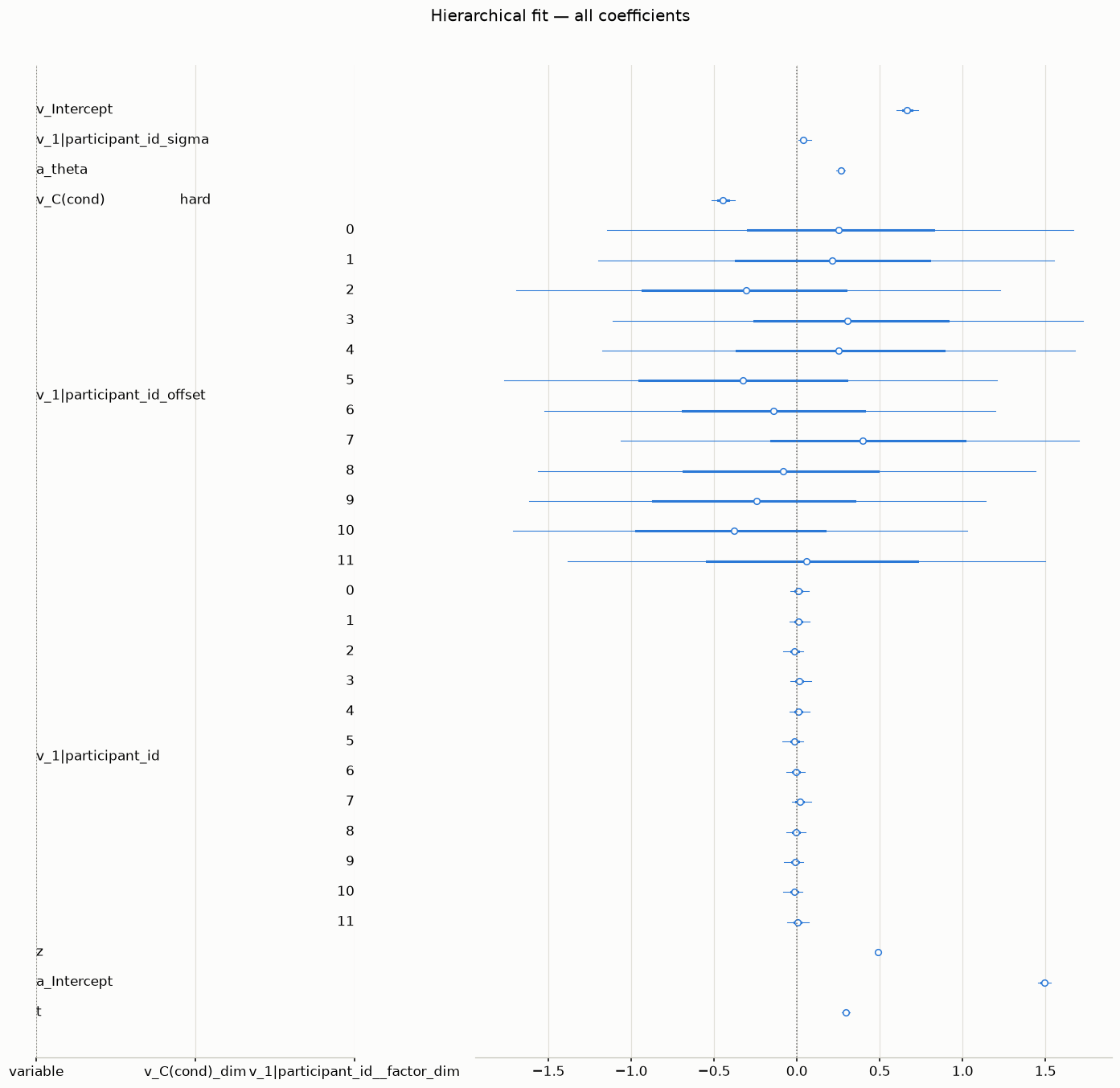
For this model the filter drops nothing: HSSM keeps the per-trial parameter values out of the posterior group and stores only the coefficients. Write the filter anyway — it costs three lines, and the moment you add a parameter that HSSM does store per trial, an unfiltered plot_forest is a figure with one row per trial.
7. Bring your own likelihood — learned from a simulator
Everything so far used a likelihood HSSM already had. For a model it has never heard of you supply one, and the contract is small:
a JAX function
f(data_i, *params) -> scalar, wheredata_iis one trial’s[rt, choice]. HSSMvmaps it over trials and differentiates it for you.
The interesting case is when there is no formula to write down — only a simulator. Then you learn the likelihood. We do it for the plain DDM on purpose: HSSM has the exact one, so we can grade the learned likelihood against the truth — the check you will not have in a real application.
The simulator, and the box it defines
ssm-simulators keeps its models in a registry that carries both the parameter names and their supported ranges. Read them out rather than hard-coding — those bounds become the region the network is valid in.
import jax.numpy as jnp
from ssms.basic_simulators.simulator import simulator
from ssms.config import model_config
from ssms.hssm_support import get_simulator_fun_internal

SIM_MODEL = "ddm"
_cfg = model_config[SIM_MODEL]
SIM_PARAMS = list(_cfg["params"])
BOX_LO = np.array(_cfg["param_bounds"][0], dtype=float)
BOX_HI = np.array(_cfg["param_bounds"][1], dtype=float)

print(f"{SIM_MODEL}: {SIM_PARAMS}")
for p, lo, hi in zip(SIM_PARAMS, BOX_LO, BOX_HI):
    print(f"  {p}: [{lo:5.2f}, {hi:5.2f}]")
ddm: ['v', 'a', 'z', 't']
v: [-3.00, 3.00]
a: [ 0.30, 2.50]
z: [ 0.10, 0.90]
t: [ 0.00, 2.00]Now a dataset at known parameters. Note the theta-shape rule from yesterday’s simulation session: a matrix of thetas with n_samples=1 gives one trial per row, which is exactly the shape a likelihood learner wants.
TRUE_SIM = dict(v=0.9, a=1.3, z=0.5, t=0.3)
N_TRIALS = 1500

_out = simulator(theta=np.tile([TRUE_SIM[p] for p in SIM_PARAMS], (N_TRIALS, 1)),
                 model=SIM_MODEL, n_samples=1, random_state=RANDOM_SEED)
sim_data = pd.DataFrame({"rt": _out["rts"].reshape(-1).astype(float),
                         "response": _out["choices"].reshape(-1).astype(float)})
print(sim_data.head(3).to_string(index=False))
print(f"\n{len(sim_data)} trials   P(+1) = {(sim_data.response > 0).mean():.3f}"
      f"   rt in [{sim_data.rt.min():.2f}, {sim_data.rt.max():.2f}]")
rt response
1.032031 1.0
1.428265 1.0
0.816103 1.0
1500 trials P(+1) = 0.909 rt in [0.42, 7.17]Training it
The simulator is fast and vectorized, so we train online — a fresh batch of \((\theta, x)\) pairs at every step, so the network never sees the same draw twice and there is nothing to overfit.
One detail worth copying. BayesFlow’s make_simulator wraps your function in a LambdaSimulator, and by default (is_batched=False) it calls that function once per sample and stacks the results. Passing is_batched=True lets us hand ssm-simulators a whole theta matrix per step — the shape rule from yesterday’s session — which is 11x faster here (2.5 ms vs 27.5 ms per batch of 128). The published BayesFlow and HSSM examples use the per-trial form.
Training takes about twenty minutes, so the notebook loads the network committed to this repository if it finds one. Set FORCE_TRAIN = True to retrain.
import os
# Must be set BEFORE keras is first imported, and must be jax: the likelihood
# has to be traceable by the sampler. (Nothing above imports keras, so this
# cell is still early enough.)
os.environ["KERAS_BACKEND"] = "jax"

import keras
import bayesflow as bf

FORCE_TRAIN = False
CKPT = pathlib.Path("checkpoints/ddm_nre.keras")

# Sizes follow BayesFlow's own examples/Ratio_Estimation.ipynb, which builds an
# NRE for this very model: a 3x256 MLP, K about half the batch, and a cosine
# decayed learning rate spanning the whole run.
EPOCHS, NUM_BATCHES, BATCH, K = 150, 300, 128, 64


def nre_sample_fn(batch_shape):
    """One fresh simulated trial per theta. x = [log rt, choice]."""
    n = int(np.prod(batch_shape))
    th = rng.uniform(BOX_LO, BOX_HI, size=(n, len(SIM_PARAMS)))
    out = simulator(theta=th, model=SIM_MODEL, n_samples=1,
                    random_state=int(rng.integers(2**31)))
    rt = out["rts"].reshape(-1).astype(np.float64)
    ch = out["choices"].reshape(-1).astype(np.float64)
    return {"theta": th.astype("float32"),
            "x": np.stack([np.log(rt), ch], -1).astype("float32")}


if CKPT.exists() and not FORCE_TRAIN:
    # NOTE: bayesflow must be imported before this, so its @serializable classes
    # are registered — otherwise the load fails with
    # "Could not locate class 'RatioApproximator'".
    approx = keras.saving.load_model(CKPT)
    print(f"loaded trained network from {CKPT}")
else:
    approx = bf.approximators.RatioApproximator(
        inference_network=bf.networks.MLP(widths=(256,) * 3),
        adapter=bf.approximators.RatioApproximator.build_adapter(
            inference_variables=["theta"],     # NRE contrasts THETA...
            inference_conditions=["x"]),       # ...against a fixed x
        standardize=["inference_variables", "inference_conditions"],
        K=K, gamma=1.0)
    approx.compile(optimizer=keras.optimizers.Adam(
        learning_rate=keras.optimizers.schedules.CosineDecay(
            5e-4, decay_steps=EPOCHS * NUM_BATCHES)))
    history = approx.fit(
        simulator=bf.make_simulator(nre_sample_fn, is_batched=True),
        epochs=EPOCHS, num_batches=NUM_BATCHES, batch_size=BATCH, verbose=2)
    bf.diagnostics.plots.loss(history)     # the one diagnostic NRE gets for free
    CKPT.parent.mkdir(parents=True, exist_ok=True)
    approx.save(CKPT)
INFO:bayesflow:Using backend 'jax'loaded trained network from checkpoints/ddm_nre.kerasFrom network to likelihood
The trained ratio is projector(classifier(...)) applied to the concatenated, standardized \((\theta, x)\). Written as a JAX function of a single trial, that is precisely HSSM’s loglik contract.
Write it as a factory that closes over the approximator, rather than as a function reaching for module globals — that is the shape HSSM’s own bayesflow_lre_integration.ipynb tutorial uses, and it means you can hold two trained networks at once without them colliding.
def make_jax_log_ratio_fn(approximator):
    """Return f(obs_i, *params) -> scalar log-ratio, ready for HSSM."""
    net, proj, std = (approximator.inference_network,
                      approximator.projector,
                      approximator.standardizer)

    def single_trial_log_ratio(data, v, a, z, t):
        theta = jnp.stack([jnp.reshape(p, ()) for p in (v, a, z, t)])
        # same transform the network was trained on
        x = jnp.stack([jnp.log(jnp.maximum(data[0], 1e-6)), data[1]])
        theta = std.maybe_standardize(theta, key="inference_variables")
        x = std.maybe_standardize(x, key="inference_conditions")
        logits = proj(net(jnp.concatenate([theta, x])[None, :]))
        return jnp.squeeze(logits).astype(jnp.float64)

    return single_trial_log_ratio


nre_logp = make_jax_log_ratio_fn(approx)
BayesFlow ships this same function, if you would rather not write it: bayesflow.wrappers.pymc.NeuralDistribution(approx, param_names=[...]) exposes it as .backend.log_prob, and wraps it as a pm.CustomDist for use in plain PyMC. We build it by hand here because we want to hand the function to HSSM and let HSSM add the parameter bounds, the non-decision-time guard and the simulator — see the next cell.
Registering it
Everything the model is — its response columns, its parameters, its density, its simulator, its validity box — goes in one call. After it, "ddm_nre" is a model name like "ddm".
# One call gives HSSM a usable random variable: it adapts the ssms simulator's
# call signature and attaches the three attributes HSSM insists on —
# `model_name`, `choices`, `obs_dim` — reading `choices` straight from the
# ssm-simulators registry. (Build it by hand and forget the attributes and you
# get "ValueError: The simulator function must have a `model_name` attribute.")
nre_rv = get_simulator_fun_internal(SIM_MODEL)
print("rv metadata:", nre_rv.model_name, nre_rv.choices, nre_rv.obs_dim)

hssm.defaults.default_model_config.pop("ddm_nre", None)   # make the cell re-runnable

hssm.register_model(
    name="ddm_nre",
    response=["rt", "response"],
    list_params=SIM_PARAMS,
    choices=[-1, 1],
    description="A DDM whose likelihood was learned from simulations by a "
                "BayesFlow ratio estimator.",
    likelihoods={
        "approx_differentiable": {
            "loglik": nre_logp,
            "backend": "jax",
            "rv": nre_rv,        # <- without this there is no posterior predictive
            # The training box, not a modelling preference. Outside it the
            # network extrapolates and returns confident nonsense.
            "bounds": dict(zip(SIM_PARAMS, zip(BOX_LO.tolist(), BOX_HI.tolist()))),
        }
    },
)
rv metadata: ddm [-1, 1] 2Declaring the density and the kind of density together, in the place that describes the model, is the point — passing loglik= and loglik_kind= to the HSSM(...) call splits one fact across two places and lets them disagree.
Now fit it, and fit the analytic DDM on the same data to grade against.
model_nre = hssm.HSSM(data=sim_data, model="ddm_nre", p_outlier=0)
model_nre.sample(sampler="numpyro", draws=500, tune=500, chains=2, cores=1,
                 random_seed=RANDOM_SEED, progressbar=False)

model_exact = hssm.HSSM(data=sim_data, model="ddm", p_outlier=0)
model_exact.sample(sampler="numpyro", draws=500, tune=500, chains=2, cores=1,
                   random_seed=RANDOM_SEED, progressbar=False)

print("LEARNED (NRE)")
print(az.summary(model_nre.traces, var_names=SIM_PARAMS, kind="stats").to_string())
print("\nEXACT (analytic WFPT)")
print(az.summary(model_exact.traces, var_names=SIM_PARAMS, kind="stats").to_string())
print("\nTRUE:", TRUE_SIM)
Model initialized successfully.INFO:hssm:Model initialized successfully.Using default initvals.
INFO:hssm:Using default initvals.

NUTS[numpyro]: [a, z, t, v]
INFO:pymc.sampling.mcmc:NUTS[numpyro]: [a, z, t, v]
We recommend running at least 4 chains for robust computation of convergence diagnostics
INFO:pymc.stats.convergence:We recommend running at least 4 chains for robust computation of convergence diagnostics
Model initialized successfully.INFO:hssm:Model initialized successfully.Using default initvals.
INFO:hssm:Using default initvals.

NUTS[numpyro]: [a, z, t, v]
INFO:pymc.sampling.mcmc:NUTS[numpyro]: [a, z, t, v]
We recommend running at least 4 chains for robust computation of convergence diagnostics
INFO:pymc.stats.convergence:We recommend running at least 4 chains for robust computation of convergence diagnostics
LEARNED (NRE)
mean sd eti89_lb eti89_ub
v 0.8 0.031 0.75 0.85
a 1.3 0.017 1.2 1.3
z 0.5 0.011 0.49 0.52
t 0.31 0.012 0.29 0.33
EXACT (analytic WFPT)
mean sd eti89_lb eti89_ub
v 0.88 0.033 0.83 0.93
a 1.3 0.021 1.3 1.3
z 0.5 0.011 0.48 0.52
t 0.3 0.012 0.28 0.31
TRUE: {'v': 0.9, 'a': 1.3, 'z': 0.5, 't': 0.3}
⚠️ p_outlier must be 0 with a ratio estimator
HSSM’s lapse process mixes the likelihood with a uniform density: \((1-p)\,\mathcal{L} + p\,\mathcal{U}\). That addition needs \(\mathcal{L}\) on a genuine probability scale, and a ratio is only defined up to the factor \(p(x)\) — so the mixture weights the two terms wrongly, silently, because nothing about the arithmetic fails.
The same rules out anything else reading the likelihood as an absolute quantity: az.loo, az.waic, and Bayes factors across separately-trained networks.
Read the two summaries together and note both things. The interval widths agree with the exact fit — the learned likelihood is not pretending to know more than the data support, which is the failure mode to fear. But v carries a small bias beyond the exact fit’s own. That is the trade: a likelihood for a model you could only simulate, at the cost of a bias you can measure but not remove.
fig, axes = plt.subplots(1, 4, figsize=(13, 3.1))
for ax, p in zip(axes, SIM_PARAMS):
    for tr, colour, lbl in [(model_exact.traces, S.PRIMARY, "exact (WFPT)"),
                            (model_nre.traces, S.NAIVE, "learned (NRE)")]:
        ax.hist(tr.posterior[p].values.ravel(), bins=40, density=True,
                color=colour, alpha=0.55, label=lbl)
    S.truth_line(ax, TRUE_SIM[p], axis="x")
    ax.set(title=p, yticks=[])
axes[0].legend(fontsize=7)
fig.suptitle("Exact vs. learned likelihood — same data, same model", y=1.04)
fig.tight_layout()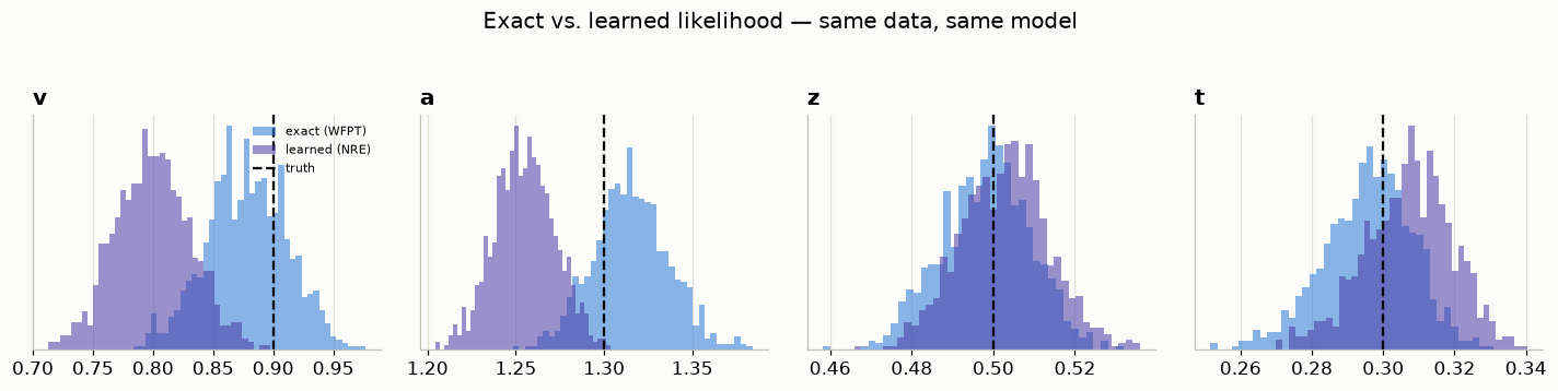
Did the sampler behave?
Same checks as for any other model — a learned likelihood buys no exemption.
az.plot_trace_dist(model_nre.traces, var_names=SIM_PARAMS, combined=False)
plt.gcf().set_size_inches(9, 6)
plt.tight_layout()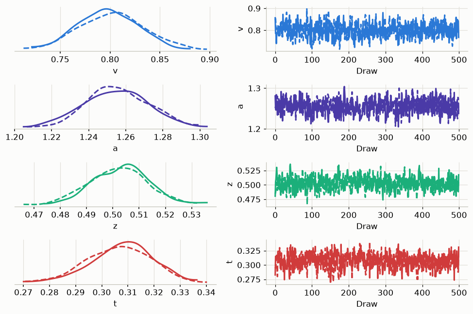
And the pair plot, which is where a custom likelihood usually confesses. Divergences are drawn on top: if they pile up in one region rather than scattering, the geometry there is the problem, not the sampler.
# ArviZ 1.x styles sub-plots through `visuals`, and divergences are OFF by
# default — you have to ask for them.
az.plot_pair(model_nre.traces, var_names=SIM_PARAMS,
             marginal=True, marginal_kind="kde",
             visuals={"divergence": True, "scatter": {"alpha": 0.1}})
plt.gcf().set_size_inches(7.5, 7.5)
plt.tight_layout()

print("divergences — learned:",
      int(model_nre.traces.sample_stats["diverging"].values.sum()),
      "  exact:", int(model_exact.traces.sample_stats["diverging"].values.sum()))
divergences — learned: 0 exact: 0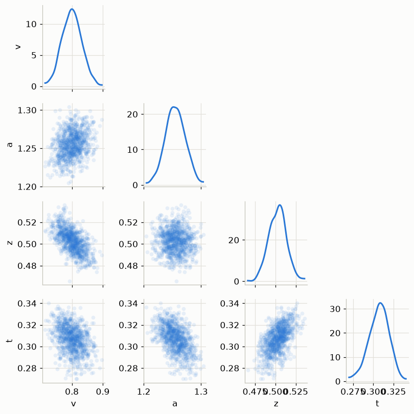
Posterior predictive
Because the registry entry carries rv=, the learned model can simulate as well as score — so HSSM’s own plots work on it, unchanged. Note we never call sample_posterior_predictive: the plot generates the draws it needs.
model_nre.plot_predictive()
plt.gcf().set_size_inches(7.5, 4)
plt.gcf().suptitle("Learned likelihood — posterior predictive vs. data", y=1.02)
plt.tight_layout()
No posterior_predictive samples found. Generating posterior_predictive samples using the provided DataTree object and the original data. This will modify the provided DataTree object, or if not provided, the traces object stored inside the model.INFO:hssm:No posterior_predictive samples found. Generating posterior_predictive samples using the provided DataTree object and the original data. This will modify the provided DataTree object, or if not provided, the traces object stored inside the model.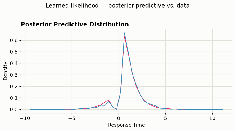
That is the whole point of registering the model properly rather than keeping the network in a variable: the likelihood is learned, but everything downstream — bounds, the lapse process, predictive sampling, the plots — is the same machinery a built-in model gets.
▶️ Which HSSM plots work for a registered custom model
plot_predictive and plot_quantile_probability are data-driven: they need the observed data and a posterior predictive, so they work for any registered model with an rv. (The quantile probability plot additionally needs a condition column to split on, which this flat single-θ dataset does not have — see section 4 for it on the conditioned dataset.)
plot_model_cartoon is the exception. It draws the latent trajectory by calling ssms.basic_simulators.simulator(model=model.model_name, …), passing the HSSM model name straight through. Our name — "ddm_nre" — means nothing to ssm-simulators, so the cartoon only works when you register under a name that package already knows.
💡 When you need a portable artifact instead
The route above hands HSSM a JAX callable, which needs nothing installed beyond what we already have — but it also means the likelihood only exists inside this Python session.
For an artifact you can ship, lanfactory.onnx.transform_bayesflow_to_onnx exports a trained approximator to ONNX, and HSSM then takes the file path directly: hssm.HSSM(..., loglik="my_net.onnx", loglik_kind="approx_differentiable"). It has real constraints — export needs KERAS_BACKEND="torch", and the network must use an identity adapter — so see HSSM’s bayesflow_nle_onnx_integration.ipynb tutorial before reaching for it.
Quick reference
| want to | call |
|---|---|
| a model | hssm.HSSM(data=df, model="ddm") |
| check what you built | print(model) · model.graph() |
| a regression on a parameter | include=[{"name": "v", "formula": "v ~ 1 + x"}] |
| participant effects | "v ~ 1 + x + (1\|participant_id)", noncentered=True |
| no lapse process | p_outlier=None |
| summarise | az.summary(model.traces, var_names=[...]) |
| SSM fit check | model.plot_quantile_probability(cond=..., predictive_style="ellipse") |
| see the process | hssm.plotting.plot_model_cartoon(model) |
| known-truth data | model.sample_do({...}, draws=1) |
| a simulator’s parameters and bounds | ssms.config.model_config["ddm"] |
| one trial per parameter row | simulator(theta=<matrix>, model="ddm", n_samples=1) |
| your own likelihood | hssm.register_model(name=..., likelihoods={"approx_differentiable": {"loglik": <jax fn>, "backend": "jax", "rv": <sim>, "bounds": ...}}) |
| learn one from simulations | bf.approximators.RatioApproximator (NRE) |
Next, at 11:00: the sigma in (1|participant_id) has a posterior geometry that will break your sampler if you let it.