MCMC for hierarchical Bayesian models

Day 3, 11:00 — 60 minutes. Alexander Fengler (with Brandon Turner).

Yesterday afternoon we saw posteriors that were hard because they were correlated — a long thin ridge, but the same shape everywhere. Hierarchical models bring a nastier relative: curvature that changes as you move. No single step size works everywhere, and the failure is not slowness. It is bias.

▶️ Running this on Google Colab

The cell below is a no-op on your own machine. On Colab it installs the stack and downloads the shared helper module, which lives one directory up in the repository and is therefore not importable there.

Expect the install to take a few minutes. If Colab asks you to restart the runtime, do it and then run the cell again — the second run is a no-op.

# --- Google Colab bootstrap; does nothing anywhere else ---------------------
import importlib.util, subprocess, sys, urllib.error, urllib.request

IN_COLAB = importlib.util.find_spec("google.colab") is not None

# `main` once this is merged; the branch is the fallback so the Colab path can
# be tested BEFORE the merge, when main does not yet have these files.
_REFS = ("main", "afengler.tutorials")
_RAW = "https://raw.githubusercontent.com/stefanradev93/sbi4cogsci/{ref}/tutorials/"


def _fetch(module):
    for ref in _REFS:
        try:
            urllib.request.urlretrieve(_RAW.format(ref=ref) + module, module)
            return ref
        except urllib.error.HTTPError:
            continue
    raise RuntimeError(f"could not fetch {module} from any of {_REFS}")


if IN_COLAB:
    # numba>=0.61 is REQUIRED, not cosmetic. pytensor resolves linker="auto" to
    # its numba backend, and numba renamed FunctionModel's first field
    # addr -> c_addr in 0.61. Colab preinstalls an older numba, and pytensor
    # declares numba only as an optional extra, so pip leaves it in place and
    # any MvNormal (SolveTriangular has no C implementation) dies with
    # KeyError: "FunctionModel does not have a field named 'c_addr'".
    subprocess.run([sys.executable, "-m", "pip", "install", "-q",
                    "numba>=0.61", "pymc>=6.2", "arviz>=1.2", "hssm>=0.4", "pymc-extras>=0.11"],
                   check=True)
    # `dot` is a system binary, not a Python package.
    subprocess.run(["apt-get", "-qq", "install", "-y", "graphviz"],
                   check=True)
    for _mod in ["sbi4cogsci_style.py", "sbi4cogsci_figures.py"]:
        print(f"  fetched {_mod} from {_fetch(_mod)}")
    print("Colab setup done.")

import sys, pathlib, warnings
sys.path.insert(0, str(pathlib.Path.cwd().parent))  # -> tutorials/

import numpy as np
import pandas as pd
import matplotlib.pyplot as plt
import pymc as pm
import arviz as az
import sbi4cogsci_style as S

S.use()
warnings.filterwarnings("ignore")

RANDOM_SEED = sum(map(ord, "sbi4cogsci-hierarchy"))
rng = np.random.default_rng(RANDOM_SEED)

DRAWS, TUNE, CHAINS = 1000, 1000, 4

print("pymc", pm.__version__, "| arviz", az.__version__)

pymc 6.2.0 | arviz 1.2.0

1. Why a hierarchy at all?

Most of this session is about a problem hierarchical models create — so first, what they buy you.

There are three options, and they are one equation with three choices of a single term. With \(G\) participants and trials \(i\) within each:

\[ p(\theta_{1:G},\, \phi \mid y) \;\propto\; \prod_{g=1}^{G} \Big[ \prod_{i} p(y_{gi} \mid \theta_g) \cdot p(\theta_g \mid \phi) \Big] \cdot p(\phi) \]

First factor the likelihood, second the population term, third the hyperprior. Every argument about pooling is an argument about the middle one:

	population term \(p(\theta_g \mid \phi)\)
complete pooling	a point mass — every \(\theta_g\) is the same \(\theta\)
no pooling	a fixed wide prior, identical and independent for each \(g\)
partial pooling	a distribution whose \(\phi\) is estimated from the data

A hierarchy is not a new inference rule — it is the ordinary posterior with one extra layer in the prior. What changes is that participants stop being independent: each estimate now depends on what the others said, through \(\phi\).

Complete pooling is what you are doing whenever you aggregate across participants and fit once, and it is wrong the moment participants differ. The other two are the interesting comparison.

Motivating setting: unbalanced data across participants. Some participants completed hundreds of trials, some barely turned up.

import sbi4cogsci_figures as F      # the shared figure module

pool = F.pooling_experiment(seed=RANDOM_SEED)
counts = pool["trial_counts"]
print(f"{counts.size} participants, {pool['n_trials_total']} trials total")
print(f"trials per participant: {counts.min()} to {counts.max()}")
print(f"  the five thinnest: {sorted(counts)[:5]}")

Initializing NUTS using jitter+adapt_diag...
Sequential sampling (4 chains in 1 job)
NUTS: [v]
Sampling 4 chains for 1_000 tune and 1_000 draw iterations (4_000 + 4_000 draws total) took 2 seconds.
Initializing NUTS using jitter+adapt_diag...
Sequential sampling (4 chains in 1 job)
NUTS: [mu_v, tau_v, z_off]
Sampling 4 chains for 1_000 tune and 1_000 draw iterations (4_000 + 4_000 draws total) took 4 seconds.

20 participants, 3081 trials total
trials per participant: 5 to 600
  the five thinnest: [np.int64(5), np.int64(6), np.int64(7), np.int64(8), np.int64(10)]

Each participant has their own drift rate, drawn from a population. We fit the same data twice, no pooling and partial pooling, and compare both against the drift rates we actually used. a, z and t are held at their true values, so the comparison is about pooling and nothing else.

summary = F.pooling_summary(pool)
print(f"{'':18s} {'MAE (all)':>10s} {'n < 30':>10s} {'n >= 30':>10s}")
for key, label in [("no_pooling", "no pooling"), ("partial_pooling", "partial pooling")]:
    d = summary[key]
    print(f"{label:18s} {d['mae_all']:10.3f} {d['mae_low']:10.3f} {d['mae_high']:10.3f}")
print(f"\nimprovement where trials < 30: {summary['low_n_improvement_pct']:.0f}%")

                    MAE (all)     n < 30    n >= 30
no pooling              0.158      0.265      0.051
partial pooling         0.114      0.175      0.052

improvement where trials < 30: 34%

F.fig_shrinkage(pool)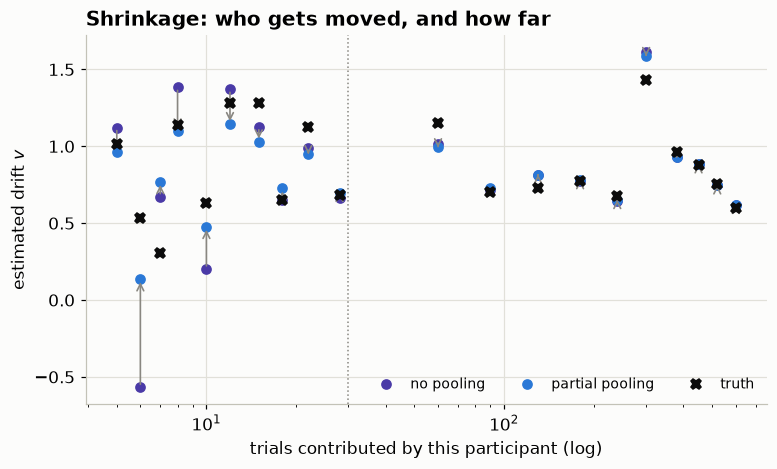

One arrow per participant, from their no-pooling estimate to their partial-pooling one. Long on the left, invisible on the right: pooling moves the participants who could not speak for themselves and leaves the rest alone.

F.fig_pooling_error(pool)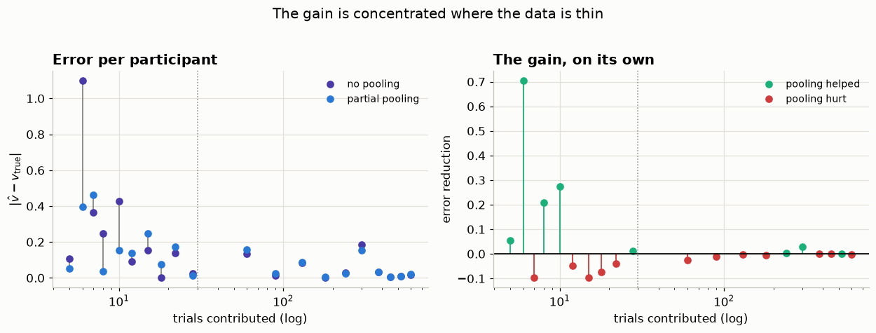

The right panel is the gain on its own: every large bar sits left of the dotted line, and past it the bars are invisible.

The red ones are the exceptions. Pooling drags each participant toward the population, which overshoots whenever one genuinely sits far from it. The guarantee is on the average — the MAE above — not on any individual.

📝 What pooling actually is

With five trials, a no-pooling estimate has almost no information, so it falls back on whatever prior you happened to write down. Partial pooling also falls back on a prior — but on the population, estimated from the participants who did have data.

Pooling replaces an arbitrary prior with an earned one. That is the whole idea, and everything after this is the price you pay for it.

Poll. Partial pooling improved the sparse participants a lot and the dense ones not at all. Why not at all?

A. The sampler converged better for them.

B. Their likelihood already dominates the prior, so shrinkage has almost nothing to pull against.

C. The population distribution does not apply to them.

D. They were closer to the population mean to begin with.

Answer

B. Shrinkage weight is roughly \(\tau^2 / (\tau^2 + \mathrm{se}_g^2)\) — it depends on how precise that participant’s own estimate is. With 600 trials the standard error is tiny, the weight goes to ~1, and the estimate barely moves. With 5 trials the standard error is large and the population wins.

Hold on to this: the same quantity decides which parameterization each group wants.

print(f"{'':18s} {'nominal':>9s} {'effective (p_loo)':>19s}")
for key, label in [("no_pooling", "no pooling"), ("partial_pooling", "partial pooling")]:
    print(f"{label:18s} {pool['nominal'][key]:9d} {pool['p_loo'][key]:19.1f}")

                     nominal   effective (p_loo)
no pooling                20                19.2
partial pooling           22                15.1

Two more nominal parameters; roughly four fewer effective ones.

A parameter costs a full unit only if the data is free to put it anywhere. Under pooling each \(v_g\) is pulled toward \(\mu\), so it is no longer free — it costs a fraction of a parameter. The two hyperparameters are not two extra freedoms; they are two knobs that remove freedom from the other twenty, and \(\tau\) is a regularisation strength learned from the data rather than guessed by you.

⚠️ Two honest caveats before you quote this number

The gap depends on how sparse your groups are. Ours has participants with five trials, and those shrink a lot. Re-run with 600 trials for everyone and the gap nearly closes: each participant’s own data identifies their drift, and p_loo approaches the nominal count. The effective-parameter story is a statement about your data, not about hierarchical models in the abstract.

elpd_loo was essentially a tie. Trial-level LOO is dominated by the participants who had plenty of trials, so it barely notices the improvement for the sparse ones. Fewer effective parameters, same trial-level predictive score — the benefit showed up in the estimates, which is what we measured before. If you care about generalising to a new participant, the matching quantity is leave-one-participant-out, not this.

📝 ArviZ 1.x naming

az.loo(idata) returns an object whose attribute is .p, although it prints as p_loo. And az.waic no longer exists — ArviZ 1.0 removed it in favour of PSIS-LOO. Nearly every tutorial you find online predates this.

2. Neal’s funnel — the geometry, before any data

Neal (2003) reduced the problem to two lines:

\[v \sim \text{Normal}(0, 3), \qquad x_i \mid v \sim \text{Normal}\!\left(0, e^{v/2}\right)\]

No data, no likelihood. This is a prior — the shape a hierarchical model has before data says anything. v is a log population scale, x a group-level parameter.

x_prior, v_prior = F.funnel_draws(n=40_000, sd_v=3.0, seed=RANDOM_SEED)
F.fig_funnel(x_prior, v_prior)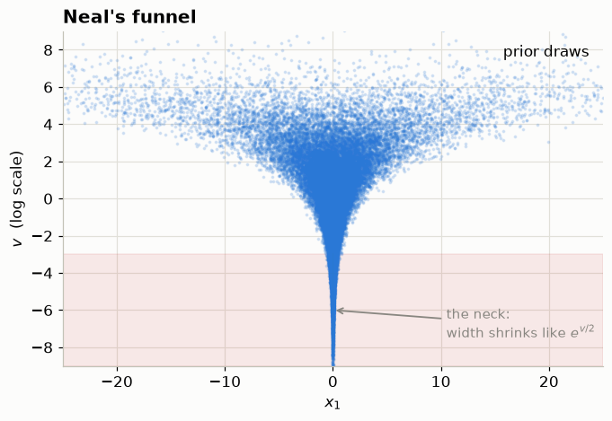

At \(v = 2\) the conditional sd of \(x\) is \(e^{1} \approx 2.7\); at \(v = -6\) it is \(e^{-3} \approx 0.05\), fifty times narrower. A step size tuned for the mouth is unstable in the neck; one tuned for the neck crawls across the mouth.

🔑 The failure mode is bias, not slowness

A sampler that cannot enter the neck does not explore it slowly — it never goes there, so every posterior expectation is wrong.

3. Sampling it, both ways

Centered — sample \(x\) directly, with its scale depending on \(v\):

\[v \sim \text{Normal}(0,3), \qquad x | v \sim \text{Normal}(0, e^{v/2})\]

Non-centered — sample a standard normal and rescale it:

\[v \sim \text{Normal}(0,3), \qquad \tilde{x} \sim \text{Normal}(0,1), \qquad x = e^{v/2}\,\tilde{x}\]

The same distribution, in two coordinate systems. The sampler only ever sees the coordinates — which is why the choice matters at all.

def funnel_centered(dim=1):
    with pm.Model() as m:
        v = pm.Normal("v", 0.0, 3.0)
        pm.Normal("x", 0.0, pm.math.exp(v / 2), shape=dim)
    return m


def funnel_noncentered(dim=1):
    with pm.Model() as m:
        v = pm.Normal("v", 0.0, 3.0)
        x_tilde = pm.Normal("x_tilde", 0.0, 1.0, shape=dim)
        pm.Deterministic("x", pm.math.exp(v / 2) * x_tilde)
    return m


def sample(model, seed=RANDOM_SEED, **kw):
    with model:
        return pm.sample(draws=DRAWS, tune=TUNE, chains=CHAINS, cores=1,
                         nuts_sampler="pymc", progressbar=False,
                         random_seed=seed, **kw)


idata_c = sample(funnel_centered())
idata_n = sample(funnel_noncentered())

for name, idata in [("centered", idata_c), ("non-centered", idata_n)]:
    div = int(idata.sample_stats["diverging"].values.sum())
    v = idata.posterior.dataset["v"].values
    print(f"{name:13s} divergences {div:5d}   "
          f"min v reached {v.min():6.2f}   mean v {v.mean():+.3f}  (true mean 0)")

Initializing NUTS using jitter+adapt_diag...
Sequential sampling (4 chains in 1 job)
NUTS: [v, x]
Sampling 4 chains for 1_000 tune and 1_000 draw iterations (4_000 + 4_000 draws total) took 1 seconds.
There were 276 divergences after tuning. Increase `target_accept` or reparameterize.
The rhat statistic is larger than 1.01 for some parameters. This indicates problems during sampling. See https://arxiv.org/abs/1903.08008 for details
The effective sample size per chain is smaller than 100 for some parameters.  A higher number is needed for reliable rhat and ess computation. See https://arxiv.org/abs/1903.08008 for details
Initializing NUTS using jitter+adapt_diag...
Sequential sampling (4 chains in 1 job)
NUTS: [v, x_tilde]
Sampling 4 chains for 1_000 tune and 1_000 draw iterations (4_000 + 4_000 draws total) took 0 seconds.

centered      divergences   276   min v reached  -3.91   mean v +0.960  (true mean 0)
non-centered  divergences     0   min v reached -11.35   mean v +0.006  (true mean 0)

The plot that shows it

fig, axes = plt.subplots(1, 2, figsize=(11.5, 4.4), sharex=True, sharey=True)
for ax, (name, idata) in zip(axes, [("centered", idata_c), ("non-centered", idata_n)]):
    post = idata.posterior.dataset
    v = post["v"].values.ravel()
    x = post["x"].values.reshape(v.size, -1)[:, 0]
    div = idata.sample_stats["diverging"].values.ravel()
    ax.plot(x, v, "o", color=S.PRIMARY, ms=2, alpha=0.25, ls="none", label="draws")
    if div.any():
        S.divergences(ax, x[div], v[div])
    ax.set(title=f"{name}  ({int(div.sum())} divergences)",
           xlabel="$x_1$", xlim=(-12, 12), ylim=(-9, 9))
    ax.legend(loc="upper right")
axes[0].set_ylabel("$v$")
fig.tight_layout()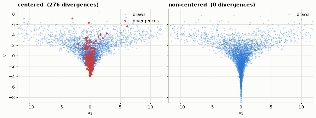

Proving it is bias

Efficiency problems shrink as you run longer. Bias does not.

fig, ax = plt.subplots(figsize=(7, 4))
for name, idata, colour in [("centered", idata_c, S.NAIVE),
                            ("non-centered", idata_n, S.PRIMARY)]:
    v = idata.posterior.dataset["v"].values[0]
    ax.plot(np.cumsum(v) / np.arange(1, v.size + 1), color=colour, label=name)
S.truth_line(ax, 0.0, label="true E[v] = 0")
ax.set(title="Running mean of $v$ (chain 0)", xlabel="draw", ylabel=r"$\hat{E}[v]$")
ax.legend()
fig.tight_layout()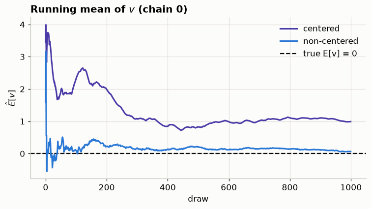

The centered chain settles at the wrong value and stays there. Running it ten times longer moves it ten times more slowly toward nothing in particular.

What about just raising target_accept?

rows = []
for ta in [0.8, 0.95, 0.99]:
    idata = sample(funnel_centered(), nuts={"target_accept": ta})
    v = idata.posterior.dataset["v"].values
    rows.append({"target_accept": ta,
                 "divergences": int(idata.sample_stats["diverging"].values.sum()),
                 "min v reached": v.min(),
                 "mean v (true 0)": v.mean()})

Initializing NUTS using jitter+adapt_diag...
Sequential sampling (4 chains in 1 job)
NUTS: [v, x]
Sampling 4 chains for 1_000 tune and 1_000 draw iterations (4_000 + 4_000 draws total) took 1 seconds.
There were 276 divergences after tuning. Increase `target_accept` or reparameterize.
The rhat statistic is larger than 1.01 for some parameters. This indicates problems during sampling. See https://arxiv.org/abs/1903.08008 for details
The effective sample size per chain is smaller than 100 for some parameters.  A higher number is needed for reliable rhat and ess computation. See https://arxiv.org/abs/1903.08008 for details
Initializing NUTS using jitter+adapt_diag...
Sequential sampling (4 chains in 1 job)
NUTS: [v, x]
Sampling 4 chains for 1_000 tune and 1_000 draw iterations (4_000 + 4_000 draws total) took 2 seconds.
There were 117 divergences after tuning. Increase `target_accept` or reparameterize.
The rhat statistic is larger than 1.01 for some parameters. This indicates problems during sampling. See https://arxiv.org/abs/1903.08008 for details
The effective sample size per chain is smaller than 100 for some parameters.  A higher number is needed for reliable rhat and ess computation. See https://arxiv.org/abs/1903.08008 for details
Initializing NUTS using jitter+adapt_diag...
Sequential sampling (4 chains in 1 job)
NUTS: [v, x]
Sampling 4 chains for 1_000 tune and 1_000 draw iterations (4_000 + 4_000 draws total) took 3 seconds.
There were 27 divergences after tuning. Increase `target_accept` or reparameterize.
The rhat statistic is larger than 1.01 for some parameters. This indicates problems during sampling. See https://arxiv.org/abs/1903.08008 for details
The effective sample size per chain is smaller than 100 for some parameters.  A higher number is needed for reliable rhat and ess computation. See https://arxiv.org/abs/1903.08008 for details

# print the table
print(pd.DataFrame(rows).to_string(index=False, float_format=lambda x: f"{x:8.3f}"))

 target_accept  divergences  min v reached  mean v (true 0)
         0.800          276         -3.914            0.960
         0.950          117         -5.752           -0.195
         0.990           27         -7.329            0.284

Divergences drop; the estimate does not become correct. Raising target_accept suppresses the symptom, not the geometry. It is a diagnostic aid. The fix is to change coordinates.

Why changing coordinates fixes it

Drop the funnel’s notation and use the hierarchy’s:

\[ \mu \sim p(\mu), \qquad \tau \sim p(\tau), \qquad \theta_g \mid \mu, \tau \sim \text{Normal}(\mu, \tau^2), \qquad y_g \mid \theta_g \sim p(y_g \mid \theta_g). \]

Centered means sampling \((\mu, \tau, \theta_1, \dots, \theta_G)\) — the parameters as written. Non-centered means sampling \((\mu, \tau, z_1, \dots, z_G)\) with

\[ z_g \sim \text{Normal}(0, 1), \qquad \theta_g = \mu + \tau z_g . \]

The map is a bijection for any fixed \(\tau > 0\), with constant Jacobian \(\partial \theta_g / \partial z_g = \tau\), so the two describe the same posterior. Nothing statistical changes. What changes is the surface the sampler walks on.

The prior term is the whole story

Write down the prior contribution in each coordinate system. Centered:

\[ \log p(\theta_g \mid \mu, \tau) = -\log \tau - \frac{(\theta_g - \mu)^2}{2\tau^2} + \text{const}. \]

That expression couples \(\theta_g\) to \(\tau\): the width of the band \(\theta_g\) may occupy is \(\tau\) — a sliver at small \(\tau\), wide at large. Plot the admissible set over \((\log \tau, \theta_g)\) and you get the funnel from section 2 — narrow neck, wide mouth.

Non-centered:

\[ \log p(z_g) = -\frac{z_g^2}{2} + \text{const}. \]

No \(\tau\). The prior geometry of \(z_g\) is a unit Gaussian whatever \(\tau\) does, so \(z\) and \(\tau\) are a priori independent and the funnel is gone — not tamed, absent. The \(\tau\)-dependence has been moved out of the geometry and into the deterministic line \(\theta_g = \mu + \tau z_g\), which the sampler never has to explore.

Why a sampler cares about the shape at all

HMC and NUTS discretise a trajectory with one step size and one mass matrix for the whole space. A step size is a claim about the scale of the distribution, and a funnel has no single scale: a step that suits the mouth overshoots the neck and the integrator diverges.

So the chain does not sample the neck badly — it fails to enter it, and every expectation comes out biased, as section 3 measured. Non-centering does not make the sampler cleverer. It hands it a space where one step size is defensible everywhere.

And why it is not free

The likelihood has been silent so far. Reinstate it, in non-centered coordinates:

\[ \log p(y_g \mid \mu + \tau z_g). \]

Now \(z_g\) and \(\tau\) appear together in the likelihood. When \(y_g\) carries real information about \(\theta_g\), it pins the product \(\mu + \tau z_g\), so raising \(\tau\) must be met by shrinking \(z_g\) — a fresh correlation, in the coordinates we adopted to remove one.

Take group \(g\) observed with standard error \(\sigma_g\), and hold \(\mu\) and \(\tau\) fixed. Prior and likelihood are both Gaussian in \(z_g\), so the conditional is too, with

\[ \operatorname{sd}(z_g \mid \tau) \;=\; \frac{\sigma_g}{\sqrt{\sigma_g^{2} + \tau^{2}}} \;\;\xrightarrow[\;\tau \gg \sigma_g\;]{}\;\; \frac{\sigma_g}{\tau} . \]

Read the two ends. When \(\tau \ll \sigma_g\) the width is \(1\) — the prior, flat in \(\tau\), which is the good case we just built. When \(\tau \gg \sigma_g\) the width pinches shut like \(1/\tau\).

A funnel again, upside down: the centered one closes at the bottom of \(\log\tau\), the non-centered one at the top. Which end you live at is decided by \(\sigma_g\) — whether group \(g\)’s own data is precise relative to how much the groups differ.

That is the whole trade:

	prior term	likelihood term	so
centered	couples \(\theta_g\) to \(\tau\) — funnel at small \(\tau\)	clean, sees \(\theta_g\) directly	good when data dominates
non-centered	independent of \(\tau\) — no funnel	couples \(z_g\) to \(\tau\) — funnel at large \(\tau\)	good when the prior dominates

Neither is correct in general.

4. Non-centered is not always better

Which one wins depends on whether the prior or the likelihood dominates each group’s posterior (Papaspiliopoulos, Roberts & Sköld 2007; Betancourt & Girolami 2013). Rather than take the crossover on faith, measure it: a hierarchical normal, swept well past it, because the far side is half the lesson.

# Two axes, not one. The NUMBER of groups is a second knob on the same geometry
# — every group adds a theta that must fit through the same neck — so the sweep
# runs at two panel sizes.
GROUP_COUNTS = [8, 24]
OBS_PER_GROUP = [1, 3, 10, 30, 100, 300, 1000]      # well past the crossover
TRUE_MU, TRUE_TAU, OBS_SIGMA = 0.0, 1.0, 1.0


def make_groups(n_groups, obs_per_group, seed):
    g = np.random.default_rng(seed)
    theta = g.normal(TRUE_MU, TRUE_TAU, n_groups)
    y = g.normal(theta[:, None], OBS_SIGMA, (n_groups, obs_per_group))
    return y.mean(axis=1), OBS_SIGMA / np.sqrt(obs_per_group)


def hier_centered(y_bar, se):
    with pm.Model() as m:
        mu = pm.Normal("mu", 0.0, 5.0)
        tau = pm.HalfNormal("tau", 5.0)
        theta = pm.Normal("theta", mu, tau, shape=y_bar.size)
        pm.Normal("y", theta, se, observed=y_bar)
    return m


def hier_noncentered(y_bar, se):
    with pm.Model() as m:
        mu = pm.Normal("mu", 0.0, 5.0)
        tau = pm.HalfNormal("tau", 5.0)
        z = pm.Normal("z", 0.0, 1.0, shape=y_bar.size)
        theta = pm.Deterministic("theta", mu + tau * z)
        pm.Normal("y", theta, se, observed=y_bar)
    return m


sweep = []
for n_groups in GROUP_COUNTS:
    for obs in OBS_PER_GROUP:
        y_bar, se = make_groups(n_groups, obs, seed=RANDOM_SEED + obs)
        for label, builder in [("centered", hier_centered),
                               ("non-centered", hier_noncentered)]:
            idata = sample(builder(y_bar, se))
            grads = idata.sample_stats["n_steps"].values.sum() \
                if "n_steps" in idata.sample_stats else np.nan
            ess = float(az.ess(idata, var_names=["tau"]).tau)
            sweep.append({"groups": n_groups, "obs/group": obs, "param": label,
                          "divergences": int(idata.sample_stats["diverging"].values.sum()),
                          "ESS(tau)": ess,
                          "ESS per 1k grads": 1000 * ess / grads if grads == grads else np.nan})

Initializing NUTS using jitter+adapt_diag...
Sequential sampling (4 chains in 1 job)
NUTS: [mu, tau, theta]
Sampling 4 chains for 1_000 tune and 1_000 draw iterations (4_000 + 4_000 draws total) took 1 seconds.
There were 236 divergences after tuning. Increase `target_accept` or reparameterize.
The rhat statistic is larger than 1.01 for some parameters. This indicates problems during sampling. See https://arxiv.org/abs/1903.08008 for details
The effective sample size per chain is smaller than 100 for some parameters.  A higher number is needed for reliable rhat and ess computation. See https://arxiv.org/abs/1903.08008 for details
Initializing NUTS using jitter+adapt_diag...
Sequential sampling (4 chains in 1 job)
NUTS: [mu, tau, z]
Sampling 4 chains for 1_000 tune and 1_000 draw iterations (4_000 + 4_000 draws total) took 1 seconds.
There were 4 divergences after tuning. Increase `target_accept` or reparameterize.
Initializing NUTS using jitter+adapt_diag...
Sequential sampling (4 chains in 1 job)
NUTS: [mu, tau, theta]
Sampling 4 chains for 1_000 tune and 1_000 draw iterations (4_000 + 4_000 draws total) took 1 seconds.
There were 15 divergences after tuning. Increase `target_accept` or reparameterize.
Initializing NUTS using jitter+adapt_diag...
Sequential sampling (4 chains in 1 job)
NUTS: [mu, tau, z]
Sampling 4 chains for 1_000 tune and 1_000 draw iterations (4_000 + 4_000 draws total) took 1 seconds.
Initializing NUTS using jitter+adapt_diag...
Sequential sampling (4 chains in 1 job)
NUTS: [mu, tau, theta]
Sampling 4 chains for 1_000 tune and 1_000 draw iterations (4_000 + 4_000 draws total) took 1 seconds.
Initializing NUTS using jitter+adapt_diag...
Sequential sampling (4 chains in 1 job)
NUTS: [mu, tau, z]
Sampling 4 chains for 1_000 tune and 1_000 draw iterations (4_000 + 4_000 draws total) took 1 seconds.
Initializing NUTS using jitter+adapt_diag...
Sequential sampling (4 chains in 1 job)
NUTS: [mu, tau, theta]
Sampling 4 chains for 1_000 tune and 1_000 draw iterations (4_000 + 4_000 draws total) took 1 seconds.
Initializing NUTS using jitter+adapt_diag...
Sequential sampling (4 chains in 1 job)
NUTS: [mu, tau, z]
Sampling 4 chains for 1_000 tune and 1_000 draw iterations (4_000 + 4_000 draws total) took 1 seconds.
There were 2 divergences after tuning. Increase `target_accept` or reparameterize.
Initializing NUTS using jitter+adapt_diag...
Sequential sampling (4 chains in 1 job)
NUTS: [mu, tau, theta]
Sampling 4 chains for 1_000 tune and 1_000 draw iterations (4_000 + 4_000 draws total) took 1 seconds.
Initializing NUTS using jitter+adapt_diag...
Sequential sampling (4 chains in 1 job)
NUTS: [mu, tau, z]
Sampling 4 chains for 1_000 tune and 1_000 draw iterations (4_000 + 4_000 draws total) took 2 seconds.
There were 10 divergences after tuning. Increase `target_accept` or reparameterize.
The rhat statistic is larger than 1.01 for some parameters. This indicates problems during sampling. See https://arxiv.org/abs/1903.08008 for details
The effective sample size per chain is smaller than 100 for some parameters.  A higher number is needed for reliable rhat and ess computation. See https://arxiv.org/abs/1903.08008 for details
Initializing NUTS using jitter+adapt_diag...
Sequential sampling (4 chains in 1 job)
NUTS: [mu, tau, theta]
Sampling 4 chains for 1_000 tune and 1_000 draw iterations (4_000 + 4_000 draws total) took 1 seconds.
Initializing NUTS using jitter+adapt_diag...
Sequential sampling (4 chains in 1 job)
NUTS: [mu, tau, z]
Sampling 4 chains for 1_000 tune and 1_000 draw iterations (4_000 + 4_000 draws total) took 3 seconds.
There were 13 divergences after tuning. Increase `target_accept` or reparameterize.
The rhat statistic is larger than 1.01 for some parameters. This indicates problems during sampling. See https://arxiv.org/abs/1903.08008 for details
The effective sample size per chain is smaller than 100 for some parameters.  A higher number is needed for reliable rhat and ess computation. See https://arxiv.org/abs/1903.08008 for details
Initializing NUTS using jitter+adapt_diag...
Sequential sampling (4 chains in 1 job)
NUTS: [mu, tau, theta]
Sampling 4 chains for 1_000 tune and 1_000 draw iterations (4_000 + 4_000 draws total) took 1 seconds.
Initializing NUTS using jitter+adapt_diag...
Sequential sampling (4 chains in 1 job)
NUTS: [mu, tau, z]
Sampling 4 chains for 1_000 tune and 1_000 draw iterations (4_000 + 4_000 draws total) took 4 seconds.
There were 13 divergences after tuning. Increase `target_accept` or reparameterize.
The rhat statistic is larger than 1.01 for some parameters. This indicates problems during sampling. See https://arxiv.org/abs/1903.08008 for details
The effective sample size per chain is smaller than 100 for some parameters.  A higher number is needed for reliable rhat and ess computation. See https://arxiv.org/abs/1903.08008 for details
Initializing NUTS using jitter+adapt_diag...
Sequential sampling (4 chains in 1 job)
NUTS: [mu, tau, theta]
Sampling 4 chains for 1_000 tune and 1_000 draw iterations (4_000 + 4_000 draws total) took 1 seconds.
There were 6 divergences after tuning. Increase `target_accept` or reparameterize.
Initializing NUTS using jitter+adapt_diag...
Sequential sampling (4 chains in 1 job)
NUTS: [mu, tau, z]
Sampling 4 chains for 1_000 tune and 1_000 draw iterations (4_000 + 4_000 draws total) took 1 seconds.
Initializing NUTS using jitter+adapt_diag...
Sequential sampling (4 chains in 1 job)
NUTS: [mu, tau, theta]
Sampling 4 chains for 1_000 tune and 1_000 draw iterations (4_000 + 4_000 draws total) took 1 seconds.
Initializing NUTS using jitter+adapt_diag...
Sequential sampling (4 chains in 1 job)
NUTS: [mu, tau, z]
Sampling 4 chains for 1_000 tune and 1_000 draw iterations (4_000 + 4_000 draws total) took 1 seconds.
Initializing NUTS using jitter+adapt_diag...
Sequential sampling (4 chains in 1 job)
NUTS: [mu, tau, theta]
Sampling 4 chains for 1_000 tune and 1_000 draw iterations (4_000 + 4_000 draws total) took 1 seconds.
Initializing NUTS using jitter+adapt_diag...
Sequential sampling (4 chains in 1 job)
NUTS: [mu, tau, z]
Sampling 4 chains for 1_000 tune and 1_000 draw iterations (4_000 + 4_000 draws total) took 1 seconds.
Initializing NUTS using jitter+adapt_diag...
Sequential sampling (4 chains in 1 job)
NUTS: [mu, tau, theta]
Sampling 4 chains for 1_000 tune and 1_000 draw iterations (4_000 + 4_000 draws total) took 1 seconds.
Initializing NUTS using jitter+adapt_diag...
Sequential sampling (4 chains in 1 job)
NUTS: [mu, tau, z]
Sampling 4 chains for 1_000 tune and 1_000 draw iterations (4_000 + 4_000 draws total) took 1 seconds.
The effective sample size per chain is smaller than 100 for some parameters.  A higher number is needed for reliable rhat and ess computation. See https://arxiv.org/abs/1903.08008 for details
Initializing NUTS using jitter+adapt_diag...
Sequential sampling (4 chains in 1 job)
NUTS: [mu, tau, theta]
Sampling 4 chains for 1_000 tune and 1_000 draw iterations (4_000 + 4_000 draws total) took 1 seconds.
Initializing NUTS using jitter+adapt_diag...
Sequential sampling (4 chains in 1 job)
NUTS: [mu, tau, z]
Sampling 4 chains for 1_000 tune and 1_000 draw iterations (4_000 + 4_000 draws total) took 2 seconds.
The rhat statistic is larger than 1.01 for some parameters. This indicates problems during sampling. See https://arxiv.org/abs/1903.08008 for details
The effective sample size per chain is smaller than 100 for some parameters.  A higher number is needed for reliable rhat and ess computation. See https://arxiv.org/abs/1903.08008 for details
Initializing NUTS using jitter+adapt_diag...
Sequential sampling (4 chains in 1 job)
NUTS: [mu, tau, theta]
Sampling 4 chains for 1_000 tune and 1_000 draw iterations (4_000 + 4_000 draws total) took 1 seconds.
Initializing NUTS using jitter+adapt_diag...
Sequential sampling (4 chains in 1 job)
NUTS: [mu, tau, z]
Sampling 4 chains for 1_000 tune and 1_000 draw iterations (4_000 + 4_000 draws total) took 2 seconds.
The rhat statistic is larger than 1.01 for some parameters. This indicates problems during sampling. See https://arxiv.org/abs/1903.08008 for details
The effective sample size per chain is smaller than 100 for some parameters.  A higher number is needed for reliable rhat and ess computation. See https://arxiv.org/abs/1903.08008 for details
Initializing NUTS using jitter+adapt_diag...
Sequential sampling (4 chains in 1 job)
NUTS: [mu, tau, theta]
Sampling 4 chains for 1_000 tune and 1_000 draw iterations (4_000 + 4_000 draws total) took 1 seconds.
Initializing NUTS using jitter+adapt_diag...
Sequential sampling (4 chains in 1 job)
NUTS: [mu, tau, z]
Sampling 4 chains for 1_000 tune and 1_000 draw iterations (4_000 + 4_000 draws total) took 3 seconds.
There were 2 divergences after tuning. Increase `target_accept` or reparameterize.
The rhat statistic is larger than 1.01 for some parameters. This indicates problems during sampling. See https://arxiv.org/abs/1903.08008 for details
The effective sample size per chain is smaller than 100 for some parameters.  A higher number is needed for reliable rhat and ess computation. See https://arxiv.org/abs/1903.08008 for details

sweep = pd.DataFrame(sweep)
for n_groups in GROUP_COUNTS:
    print(f"\n--- {n_groups} groups " + "-" * 44)
    print(sweep[sweep.groups == n_groups].drop(columns="groups")
          .to_string(index=False, float_format=lambda x: f"{x:9.2f}"))

--- 8 groups --------------------------------------------
 obs/group        param  divergences  ESS(tau)  ESS per 1k grads
         1     centered          236     15.41              0.38
         1 non-centered            4    906.91             21.12
         3     centered           15   1969.23             72.26
         3 non-centered            0    948.44             23.50
        10     centered            0   3224.16            121.75
        10 non-centered            0    686.19             13.14
        30     centered            0   3919.49            151.61
        30 non-centered            2    662.00             10.21
       100     centered            0   3498.52            139.22
       100 non-centered           10    316.76              2.87
       300     centered            0   3410.09            140.75
       300 non-centered           13    398.06              2.23
      1000     centered            0   3935.28            159.89
      1000 non-centered           13    340.54              1.43

--- 24 groups --------------------------------------------
 obs/group        param  divergences  ESS(tau)  ESS per 1k grads
         1     centered            6    556.09             11.85
         1 non-centered            0    966.94             24.91
         3     centered            0   4305.97            154.05
         3 non-centered            0   1060.39             30.33
        10     centered            0   4559.33            163.00
        10 non-centered            0    916.33             27.44
        30     centered            0   8129.98            291.40
        30 non-centered            0    572.20              8.77
       100     centered            0   8258.80            296.18
       100 non-centered            0    292.54              3.56
       300     centered            0   8258.49            296.77
       300 non-centered            0    162.74              1.66
      1000     centered            0   7773.29            278.97
      1000 non-centered            2    158.87              1.14

fig, (ax1, ax2) = plt.subplots(1, 2, figsize=(11.5, 4.1))
for label, colour in [("centered", S.NAIVE), ("non-centered", S.PRIMARY)]:
    for n_groups, style in zip(GROUP_COUNTS, ["-", "--"]):
        sub = sweep[(sweep.param == label) & (sweep.groups == n_groups)]
        tag = f"{label}, {n_groups} groups"
        ax1.plot(sub["obs/group"], sub["divergences"], "o" + style, color=colour,
                 label=tag, ms=5)
        ax2.plot(sub["obs/group"], sub["ESS per 1k grads"], "o" + style,
                 color=colour, label=tag, ms=5)
ax1.set(title="Divergences", xlabel="observations per group", xscale="log",
        yscale="symlog", ylabel="count")
ax1.legend(fontsize=8)
ax2.set(title="Efficiency", xlabel="observations per group", xscale="log",
        yscale="log", ylabel=r"ESS($\tau$) per 1k gradients")
ax2.legend(fontsize=8)
fig.tight_layout()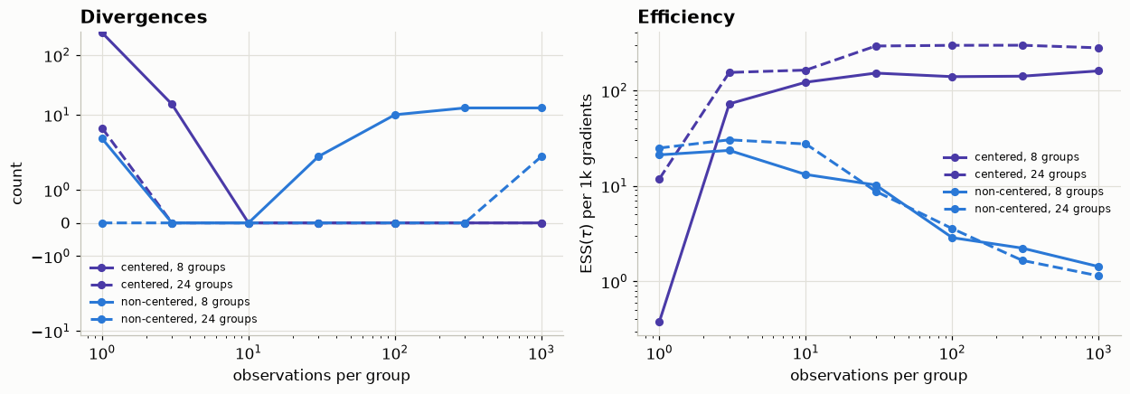

Read the right-hand panel first, and note the log vertical axis. The two curves cross almost immediately — non-centered wins only in the sparsest column, at one observation per group — and then separate: by 1000 observations per group, centering is worth a hundredfold to two-hundredfold difference in ESS per unit of work, depending on panel size. The far end of this sweep is not a curiosity; it is where a lot of real cognitive data sits.

📝 The rule, stated properly

“Always non-center hierarchical models” is the single most widespread piece of wrong advice in applied Bayesian work. The correct statement is: non-center the parameters whose groups are data-poor.

Which is why you want the choice to be per parameter.

🔑 More groups suppresses the divergences without fixing the efficiency

Compare the solid lines (8 groups) with the dashed ones (24). Divergences largely disappear on the bigger panel: the centered fit at one observation per group falls from 236 divergences to 6, and the non-centered fit’s complaints at the data-rich end (10, 13, 13) drop to (0, 0, 2).

That is not the geometry being repaired. It is Betancourt’s remark, now readable off a figure: more groups means more information about \(\tau\), which trims off the extreme values of \(\tau\) where the pathology lives.

The efficiency panel keeps its shape and its ordering throughout. So a clean divergence count is not evidence you chose the right parameterization — only that you had enough groups to hide the wrong one. Judge by ESS per gradient, and let divergences tell you about correctness rather than about cost.

What that looks like in the geometry

The ESS curves say that the advantage reverses; this says why. Four fits — both parameterizations, at weak and strong data — each in the coordinates its own sampler works in, against \(\log\tau\), divergences overlaid. Rubin’s eight schools, unmodified.

Two details of the setup are load-bearing; get either wrong and the bottom-right panel looks harmless when it is not.

Which group gets plotted. The non-centered ridge is \(z_g = (y_g - \mu)/\tau\), so its slope against \(\log\tau\) is \(-z_g\) — a group sitting near the population mean draws a flat blob however bad the geometry is. We plot the group furthest from the mean, chosen from the data so that both columns show the same school.

The prior on \(\tau\). HalfNormal(25), not the customary HalfNormal(5). The schools’ effects run to 28 points and the strong-likelihood posterior for \(\tau\) sits near 10, so a scale of 5 truncates \(\tau\)’s upper tail — which is exactly where the non-centered form pinches. Same data, same code, that one number changed: 2 divergences becomes 88, while the centered fit reports zero either way. A prior tight enough to hide a pathology is not weakly informative, whatever it says on the tin.

geom = F.geometry_experiment(seed=RANDOM_SEED)
print(f"{geom['n_groups']} groups")
F.fig_geometry_grid(geom)

Initializing NUTS using jitter+adapt_diag...
Sequential sampling (4 chains in 1 job)
NUTS: [mu, tau, theta]
Sampling 4 chains for 2_000 tune and 2_000 draw iterations (8_000 + 8_000 draws total) took 2 seconds.
There were 466 divergences after tuning. Increase `target_accept` or reparameterize.
The rhat statistic is larger than 1.01 for some parameters. This indicates problems during sampling. See https://arxiv.org/abs/1903.08008 for details
The effective sample size per chain is smaller than 100 for some parameters.  A higher number is needed for reliable rhat and ess computation. See https://arxiv.org/abs/1903.08008 for details
Initializing NUTS using jitter+adapt_diag...
Sequential sampling (4 chains in 1 job)
NUTS: [mu, tau, z]
Sampling 4 chains for 2_000 tune and 2_000 draw iterations (8_000 + 8_000 draws total) took 2 seconds.
There were 36 divergences after tuning. Increase `target_accept` or reparameterize.
Initializing NUTS using jitter+adapt_diag...
Sequential sampling (4 chains in 1 job)
NUTS: [mu, tau, theta]
Sampling 4 chains for 2_000 tune and 2_000 draw iterations (8_000 + 8_000 draws total) took 1 seconds.
Initializing NUTS using jitter+adapt_diag...
Sequential sampling (4 chains in 1 job)
NUTS: [mu, tau, z]
Sampling 4 chains for 2_000 tune and 2_000 draw iterations (8_000 + 8_000 draws total) took 6 seconds.
There were 88 divergences after tuning. Increase `target_accept` or reparameterize.

8 groups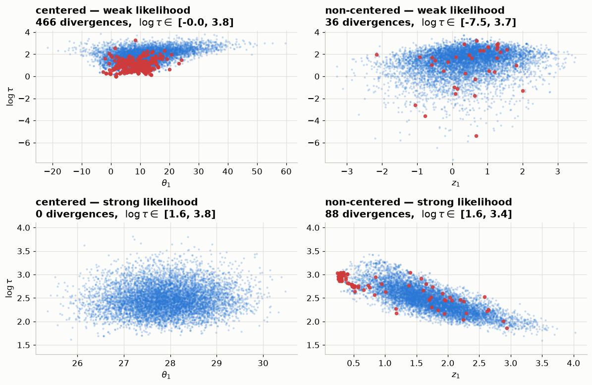

print(f"{'parameterization':16s} {'se scale':>9s} {'divergences':>12s} "
      f"{'log tau reached':>17s} {'ESS(tau)':>10s} {'corr w/ log tau':>16s}")
for (scale, par), d in geom["results"].items():
    span = f"{d['min_log_tau']:6.2f} .. {d['max_log_tau']:5.2f}"
    print(f"{par:16s} {scale:9g} {d['n_divergences']:12d} "
          f"{span:>17s} {d['ess_tau']:10.1f} {d['corr']:16.2f}")

parameterization  se scale  divergences   log tau reached   ESS(tau)  corr w/ log tau
centered                 1          466    -0.01 ..  3.84      135.6             0.37
non-centered             1           36    -7.52 ..  3.72     2575.2             0.20
centered              0.05            0     1.62 ..  3.81     7011.2             0.07
non-centered          0.05           88     1.60 ..  3.43      820.6            -0.78

The two panels in each row share a \(\log\tau\) axis — that is what makes the comparison honest.

Top row (weak likelihood). The centered chain simply stops at \(\log\tau \approx 0\), with hundreds of divergences piled against that floor, and reports \(\hat{R} \approx 1\) while doing it. The non-centered chain, on the same axis, carries on down past \(-7\).

Bottom row (strong likelihood). Everything swaps, and this is the panel to look at hardest. Centered collapses to a round blob: the data pins \(\theta_1\) near 28, \(\tau\) has stopped mattering to it, correlation +0.07, zero divergences. Non-centered has bent into a curved band with correlation −0.78 — that is \(z_1 = (y_1 - \mu)/\tau\) traced out as \(\tau\) moves, the coupling we changed coordinates to get rid of, back again. It throws 88 divergences, and they are not scattered: they sit at the 87th percentile of \(\log\tau\), piled against the top of the band exactly as the centered chain’s pile against the bottom of the neck. It also stops climbing at \(\log\tau = 3.4\) where the centered chain reaches \(3.8\).

That is section 3’s trade table, measured: the same pathology in the opposite corner of the grid, at the opposite end of \(\tau\). In both rows the tell is identical — the failing chain cannot reach where the healthy one goes.

📝 Why the bottom-right band does not visibly taper

The derivation says \(\operatorname{sd}(z_g \mid \tau) \to \sigma_g/\tau\), so you might expect that band to close like a wedge. It does not — measured across quartiles of \(\log\tau\), its width is 0.46, 0.37, 0.37, 0.39.

Because the panel is a marginal, and \(\mu\) is free in it. With \(z_g = (\theta_g - \mu)/\tau\) and \(\mu\) carrying posterior sd \(\tau/\sqrt{G}\), \(\mu\) alone contributes \(1/\sqrt{G} = 0.35\) to the width of \(z_g\) — the same at every \(\tau\). The \(\sigma_g/\tau\) pinch runs from 0.15 down to 0.02 underneath that and is simply swamped.

The conditional funnel is real and it is what the sampler feels. The marginal shows it as curvature and correlation instead of as a taper. Worth remembering generally: a 2-D marginal is not the geometry, it is a shadow of it.

📝 Why the panel is eight groups

Because the group count only affects one of the two pathologies, and in the direction that hides it — the effect the sweep’s divergence panel showed above, now playing out on the other parameterization.

Re-run the whole grid at 8 / 16 / 32 / 64 groups. The centered fit under a weak likelihood barely notices (466, 309, 343, 77 divergences). The non-centered fit under a strong likelihood does this:

groups	8	16	32	64
divergences	88	21	2	0
ESS(\(\tau\))	821	565	311	163

The divergences vanish while the efficiency gets five times worse. More groups does not repair the geometry; it pins \(\tau\) and removes the extreme values that expose it — Betancourt’s “the pathological behavior is the worst exactly when the partial pooling is strongest.”

Eight groups is where the reversal costs you correctness, which is why the figure uses eight. At the group counts you will actually have, expect it to cost you silently.

⚠️ Do not memorise the crossover point

The crossover moves with the number of groups, the group-scale prior, and how much the groups actually differ — so “the crossover is between 1 and 3 observations per group” is a fact about this setup, not a constant. You saw two of those dependencies measured on this page: the panel size took the non-centered divergence count from 88 to 0, and the prior scale on \(\tau\) took it from 2 to 88.

What transfers is the shape: two curves that cross, and a rule for which side you are on. Run the sweep on your own model rather than importing a number from someone else’s.

5. Per-parameter parameterization in HSSM

A real SSM has parameters of both kinds in the same model. Drift v is often estimated from plenty of trials per participant; a boundary or non-decision time may be far more weakly identified. HSSM lets you choose independently.

import hssm

data = hssm.load_data("cavanagh_theta")
print(data.head(3).to_string(index=False))
print("\nparticipants:", data["participant_id"].nunique(), " trials:", len(data))

 participant_id stim   rt  response     theta  dbs conf
              0   LL 1.21       1.0  0.656275    1   HC
              0   WL 1.63       1.0 -0.327889    1   LC
              0   WW 1.03       1.0 -0.480285    1   HC

participants: 14  trials: 3988

noncentered is not an HSSM argument — it passes straight through to bmb.Model. It takes a bool or a dict keyed by parameter, and a per-prior setting overrides the dict:

resolution order:  prior.noncentered  >  noncentered[param]  >  True

mixed = hssm.HSSM(
    data=data,
    model="ddm",
    noncentered={"v": False, "a": True},
    include=[
        {"name": "v", "formula": "v ~ 1 + (1|participant_id)"},
        {"name": "a", "formula": "a ~ 1 + (1|participant_id)"},
    ],
    p_outlier=0.05,          # explicit: this is the default, not "off"
    prior_settings="safe",
)

# The PyMC graph is materialised at construction — no `.build()` to call.
participant_nodes = sorted(n for n in mixed.pymc_model.named_vars
                           if "participant_id" in n)
print("participant-level nodes:")
for n in participant_nodes:
    mark = "  <- non-centered" if n.endswith("_offset") else ""
    print(f"    {n}{mark}")

Model initialized successfully.
participant-level nodes:
    a_1|participant_id
    a_1|participant_id_offset  <- non-centered
    a_1|participant_id_sigma
    v_1|participant_id
    v_1|participant_id_sigma

The _offset nodes are the structural fingerprint of the non-centered parameterization: u_g = z_g · σ. a has one, v does not — read off the graph, without sampling anything.

⚠️ Two ways this bites

Non-centering only works for Normal priors whose sigma is itself a random variable:

Anything else raises NotImplementedError when the model is built — loud, at least.

Check for disconnected nodes:

A Normal group prior with a nested mu hyperprior under non-centering leaves mu as a disconnected free variable — sampled, but influencing nothing. HSSM 0.4.0 ships detectors for this (check_user_priors_against_parameterization, find_disconnected_free_rvs). Always check print(model) / model.graph() after changing parameterization, because term-prior keys differ between the two forms and a mismatched key is silently dropped.

Where per-parameter runs out

The choice is per random effect, so every group inside one effect gets the same treatment — and groups can disagree. Betancourt’s example: nine groups with \(N = (10, 5, \mathbf{1000}, 10, 1, 5, \mathbf{100}, 10, 5)\). Center everything and the sparse groups funnel; non-center everything and the two rich ones inverted-funnel. The right answer there is per group, which no API on this page exposes.

And it is quiet. Both monolithic fits on that panel diverge at rates of 0.015% and 0.005% — a handful out of thousands, the kind you would wave away. The aggregate count averages over groups, and two broken groups out of nine do not move it. You find them the way section 4 did: plot \(\theta_g\) or \(z_g\) against \(\log\tau\) one group at a time.

The fix — split the groups at a size threshold and parameterize each half its own way — needs per-group surgery on the model.

Exercise

Build the same model with noncentered=True and with noncentered=False, and confirm from the graph alone (no sampling) which nodes change. Then predict — before running anything — which setting you would want for v in the Cavanagh data, given its 3,988 trials spread over 14 participants.

Solution and reasoning

for setting in [True, False]:
    m = hssm.HSSM(
        data=data, model="ddm", noncentered=setting,
        include=[{"name": "v", "formula": "v ~ 1 + (1|participant_id)"}],
        p_outlier=0.05, prior_settings="safe",
    )
    offs = sorted(n for n in m.pymc_model.named_vars if n.endswith("_offset"))
    print(setting, "->", offs)

With roughly 285 trials per participant, the drift rate is well identified within each participant — the likelihood dominates, so centered is the better choice for v. Parameters that are weakly constrained per participant, or a group scale estimated from only 14 groups, are the ones that want non-centering. This is the crossover from section 4, in a real model.

References

• Neal, R. (2003). Slice sampling. Annals of Statistics 31(3), 705–767.
• Papaspiliopoulos, Roberts & Sköld (2007). A general framework for the parametrization of hierarchical models. Statistical Science 22(1), 59–73.
• Betancourt & Girolami (2013). Hamiltonian Monte Carlo for hierarchical models. arXiv:1312.0906 — the source of the weak/strong likelihood manipulation used in the geometry grid.
• Betancourt (2017). Diagnosing biased inference with divergences.
• Betancourt (2020). Hierarchical modeling — the long-form version of section 4, including why the prior on \(\tau\) has to be chosen so that it does not hide the geometry.
• Gorinova, Moore & Hoffman (2020). Automatic reparameterisation of probabilistic programs. ICML.