Hierarchical modelling from scratch: the alien coins

Day 3 — companion notebook. Brandon Turner, Alexander Fengler.

A Python version of binomial_Bayes_hier.R. We write the sampler by hand first — it is about thirty lines of numpy — and only then call PyMC, so the library is doing something you have already seen.

The example is the one from the slides: alien coins, each with some magnetic property that pushes \(P(\text{heads})\) away from \(0.5\) by a different amount. Flip each one a fixed number of times, estimate each one’s bias.

The same question, asked three ways:

	what you assume	what you get
no pooling	every coin is unrelated	each coin’s own flips, and nothing else
fixed population	coins share a population you already know	shrinkage toward a known centre
hierarchical	coins share a population you must also estimate	shrinkage, plus the population itself

The third is the one worth the trouble. What it buys and what it costs is the whole content of this notebook.

▶️ Running this on Google Colab

The cell below is a no-op on your own machine. On Colab it installs the stack and downloads the shared helper module, which lives one directory up in the repository and is therefore not importable there.

Expect the install to take a few minutes. If Colab asks you to restart the runtime, do it and then run the cell again — the second run is a no-op.

# --- Google Colab bootstrap; does nothing anywhere else ---------------------
import importlib.util, subprocess, sys, urllib.error, urllib.request

IN_COLAB = importlib.util.find_spec("google.colab") is not None

_REFS = ("main", "af-reductions-toy-models")
_RAW = "https://raw.githubusercontent.com/stefanradev93/sbi4cogsci/{ref}/tutorials/"


def _fetch(module):
    for ref in _REFS:
        try:
            urllib.request.urlretrieve(_RAW.format(ref=ref) + module, module)
            return ref
        except urllib.error.HTTPError:
            continue
    raise RuntimeError(f"could not fetch {module} from any of {_REFS}")


if IN_COLAB:
    # numba>=0.61 is REQUIRED, not cosmetic. pytensor resolves linker="auto" to
    # its numba backend, and numba renamed FunctionModel's first field
    # addr -> c_addr in 0.61. Colab preinstalls an older numba, and pytensor
    # declares numba only as an optional extra, so pip leaves it in place.
    subprocess.run([sys.executable, "-m", "pip", "install", "-q",
                    "numba>=0.61", "pymc>=6.2", "arviz>=1.2"], check=True)
    for _mod in ["sbi4cogsci_style.py"]:
        print(f"  fetched {_mod} from {_fetch(_mod)}")
    print("Colab setup done.")

import sys, pathlib, warnings

sys.path.insert(0, str(pathlib.Path.cwd().parent))  # -> tutorials/

import numpy as np
import matplotlib.pyplot as plt
from scipy import stats
import pymc as pm
import arviz as az
import sbi4cogsci_style as S

S.use()
warnings.filterwarnings("ignore")

RANDOM_SEED = sum(map(ord, "sbi4cogsci-alien-coins"))
rng = np.random.default_rng(RANDOM_SEED)

print("pymc", pm.__version__, "| arviz", az.__version__)

pymc 6.2.0 | arviz 1.2.0

1. The coins, and where they come from

The generative story, exactly as the slides draw it:

\[ \alpha,\ \beta \quad\longrightarrow\quad p_i \sim \text{Beta}(\alpha, \beta) \quad\longrightarrow\quad D_i \sim \text{Bernoulli}(p_i)\ \ (n \text{ flips}). \]

Downward it is a recipe for making data. Upward it is the inference problem: from \(D\), recover every \(p_i\) and the \(\alpha, \beta\) behind them.

We simulate, so everything later is checkable against a known truth.

N_FLIPS = 100          # flips per coin
S_COINS = 24           # number of coins
TRUE_ALPHA, TRUE_BETA = 10.0, 15.0

true_p = rng.beta(TRUE_ALPHA, TRUE_BETA, size=S_COINS)
data = rng.binomial(1, true_p[:, None], size=(S_COINS, N_FLIPS))   # 0/1 flips
x = data.sum(axis=1)                                               # heads per coin

pop_mean = TRUE_ALPHA / (TRUE_ALPHA + TRUE_BETA)
print(f"population mean = alpha/(alpha+beta) = {pop_mean:.3f}")
print(f"true p ranges {true_p.min():.3f} to {true_p.max():.3f}")
print(f"heads out of {N_FLIPS}: {x}")

population mean = alpha/(alpha+beta) = 0.400
true p ranges 0.199 to 0.587
heads out of 100: [31 34 33 32 61 31 40 31 19 30 34 56 42 46 31 35 54 27 44 42 40 32 43 37]

fig, (ax1, ax2) = plt.subplots(1, 2, figsize=(11, 3.6))

grid = np.linspace(0, 1, 400)
ax1.plot(grid, stats.beta.pdf(grid, TRUE_ALPHA, TRUE_BETA), color=S.PRIMARY,
         lw=2, label=rf"Beta({TRUE_ALPHA:.0f}, {TRUE_BETA:.0f})")
ax1.plot(true_p, np.zeros_like(true_p), "|", color=S.TRUTH, ms=14,
         label="the 24 true $p_i$")
ax1.set(title="The population the coins were drawn from", xlabel="$p$",
        ylabel="density", xlim=(0, 1))
ax1.legend(fontsize=9)

ax2.plot(true_p, x / N_FLIPS, "o", color=S.PRIMARY, ms=6, ls="none")
lims = (0, 0.9)
ax2.plot(lims, lims, "--", color=S.TRUTH, lw=1.5, label="perfect")
ax2.set(title="What 100 flips tell you about each coin", xlabel="true $p_i$",
        ylabel="observed proportion", xlim=lims, ylim=lims)
ax2.legend(fontsize=9)
fig.tight_layout()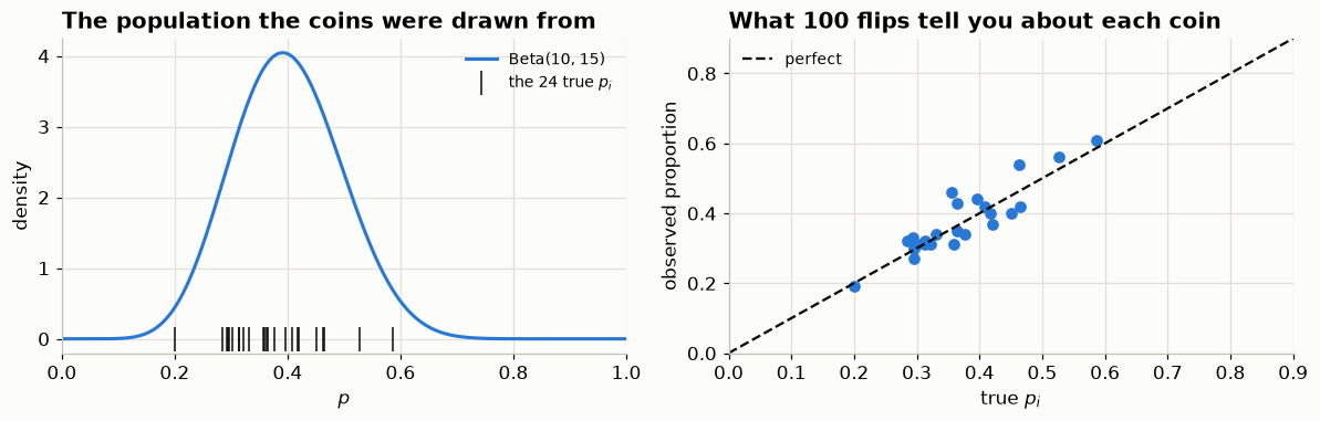

The right panel is the no-pooling estimate — each coin’s own proportion of heads and nothing else. It scatters around the truth with no systematic bias.

Keep that in mind, because next we make it biased on purpose and end up closer to the truth.

2. One coin, by hand

One coin, and the three pieces the R script writes: a likelihood, a prior, their product. In logs — a product of 100 probabilities underflows fast.

def log_lik(p, flips):
    """log P(flips | p) for one coin. Bernoulli, summed over flips."""
    if not (0.0 < p < 1.0):
        return -np.inf
    return float(np.sum(stats.bernoulli.logpmf(flips, p)))


def log_prior(p, alpha, beta):
    """log Beta(p | alpha, beta) — the population, seen from one coin."""
    return float(stats.beta.logpdf(p, alpha, beta))


def log_post(p, flips, alpha, beta):
    """Unnormalised log posterior. -inf outside the support, as in the R."""
    out = log_lik(p, flips) + log_prior(p, alpha, beta)
    return -np.inf if np.isnan(out) else out


coin = 0
print(f"coin {coin}: {x[coin]} heads out of {N_FLIPS}   (true p = {true_p[coin]:.3f})")
print(f"  log-likelihood at p = 0.4 : {log_lik(0.4, data[coin]):.3f}")
print(f"  log-prior      at p = 0.4 : {log_prior(0.4, TRUE_ALPHA, TRUE_BETA):.3f}")
print(f"  log-posterior  at p = 0.4 : {log_post(0.4, data[coin], TRUE_ALPHA, TRUE_BETA):.3f}")

coin 0: 31 heads out of 100   (true p = 0.302)
  log-likelihood at p = 0.4 : -63.652
  log-prior      at p = 0.4 : 1.394
  log-posterior  at p = 0.4 : -62.258

One parameter, so we can just look at the posterior on a grid. Worth doing once: this is the thing MCMC approximates once a grid stops being an option.

ps = np.linspace(0.001, 0.999, 400)
lp_like = np.array([log_lik(p, data[coin]) for p in ps])
lp_prior = np.array([log_prior(p, TRUE_ALPHA, TRUE_BETA) for p in ps])
lp_post = lp_like + lp_prior


def to_density(logs):
    """Exponentiate a log-density safely and normalise it for plotting."""
    d = np.exp(logs - logs.max())
    return d / np.trapezoid(d, ps)


fig, ax = plt.subplots(figsize=(7.5, 4.0))
ax.plot(ps, to_density(lp_prior), color=S.ALT, lw=2, label="prior — the population")
ax.plot(ps, to_density(lp_like), color=S.NAIVE, lw=2, label="likelihood — this coin's flips")
ax.plot(ps, to_density(lp_post), color=S.PRIMARY, lw=2.5, label="posterior — both")
S.truth_line(ax, true_p[coin], axis="x", label=f"true $p_{{{coin}}}$")
ax.set(title=f"Coin {coin}: {x[coin]} heads in {N_FLIPS} flips", xlabel="$p$",
       ylabel="density", xlim=(0, 1))
ax.legend(fontsize=9)
fig.tight_layout()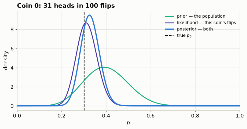

The posterior sits between the likelihood and the prior, nearer whichever is sharper. That is pooling, already visible before any hierarchy exists: the population pulls the estimate toward it, by an amount that depends on how much this coin’s own data has to say.

3. Method 1 — sample every coin, with the population known

Now all 24 coins at once, with a Metropolis sampler written out. This is a direct translation of the first sampler in the R script: a symmetric normal proposal, an accept/reject on the log-posterior ratio, and one chain per coin advancing in lockstep.

Note that it assumes \(\alpha\) and \(\beta\) are known and plugs in the true values. That is cheating; section 5 removes it. One idea at a time, which is why the R script goes in this order.

def metropolis_known_pop(alpha, beta, n_iter=2000, tune=0.05, seed=RANDOM_SEED):
    """One Metropolis chain per coin. alpha/beta fixed and given."""
    rng_m = np.random.default_rng(seed)
    p_chain = np.empty((n_iter, S_COINS))
    lp = np.empty(S_COINS)

    p_chain[0] = rng_m.beta(1.0, 1.0, S_COINS)      # "your guess is as good as mine"
    for j in range(S_COINS):
        lp[j] = log_post(p_chain[0, j], data[j], alpha, beta)

    n_acc = np.zeros(S_COINS)
    for t in range(1, n_iter):
        prop = rng_m.normal(p_chain[t - 1], tune)    # symmetric -> ratio is the whole rule
        for j in range(S_COINS):
            lp_prop = log_post(prop[j], data[j], alpha, beta)
            if np.log(rng_m.uniform()) < lp_prop - lp[j]:
                p_chain[t, j], lp[j], n_acc[j] = prop[j], lp_prop, n_acc[j] + 1
            else:
                p_chain[t, j] = p_chain[t - 1, j]
    return p_chain, n_acc / (n_iter - 1)


chain_known, acc_known = metropolis_known_pop(TRUE_ALPHA, TRUE_BETA)
print(f"acceptance rate: mean {acc_known.mean():.2f}, "
      f"range {acc_known.min():.2f}-{acc_known.max():.2f}")

acceptance rate: mean 0.66, range 0.64-0.69

WARMUP = 500
post_known = chain_known[WARMUP:]

fig, axes = plt.subplots(2, 3, figsize=(12, 5.2))
for k, j in enumerate([0, 1, 2]):
    ax = axes[0, k]
    ax.plot(chain_known[:, j], lw=0.6, color=S.PRIMARY)
    S.truth_line(ax, true_p[j], label="truth")
    ax.set(title=f"coin {j}", xlabel="iteration", ylabel="$p$", ylim=(0, 1))
    if k == 0:
        ax.legend(fontsize=8)

    ax = axes[1, k]
    ax.hist(post_known[:, j], bins=30, density=True, color=S.PRIMARY, alpha=0.75)
    S.truth_line(ax, true_p[j], axis="x")
    ax.set(xlabel="$p$", ylabel="density", xlim=(0, 1))
fig.suptitle("Method 1 — traces (top) and posteriors (bottom), population known",
             y=1.01)
fig.tight_layout()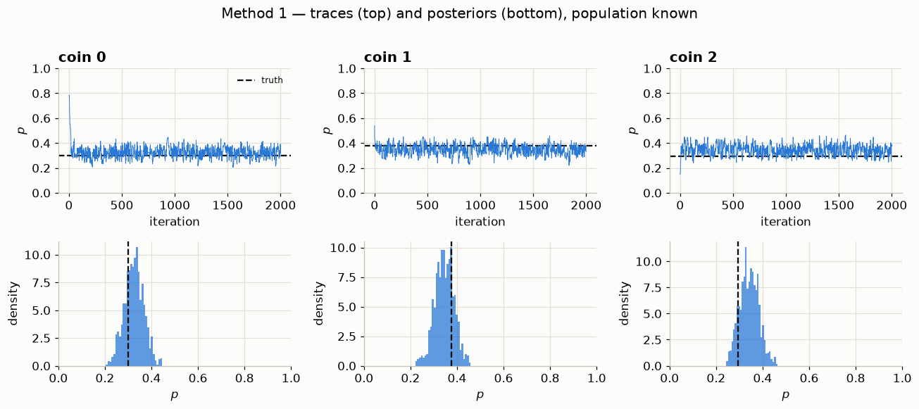

The chains leave their random starting points, settle, and wander around the truth. The R script draws this for all 24 coins in a loop; three is enough.

The summary that matters is every coin at once, estimate against truth.

est_known = post_known.mean(axis=0)
naive = x / N_FLIPS


def recovery_panel(ax, est, title, colour):
    ax.plot(true_p, est, "o", color=colour, ms=6, ls="none")
    lims = (0.05, 0.85)
    ax.plot(lims, lims, "--", color=S.TRUTH, lw=1.5)
    S.truth_line(ax, pop_mean, axis="x", label="population mean")
    rmse = np.sqrt(np.mean((est - true_p) ** 2))
    ax.set(title=f"{title}\nRMSE = {rmse:.4f}", xlabel="true $p_i$",
           ylabel="estimate", xlim=lims, ylim=lims)
    return rmse


fig, (ax1, ax2) = plt.subplots(1, 2, figsize=(10.5, 4.4))
rmse_naive = recovery_panel(ax1, naive, "No pooling (each coin alone)", S.NAIVE)
rmse_known = recovery_panel(ax2, est_known, "Population known", S.PRIMARY)
ax2.legend(fontsize=8, loc="upper left")
fig.tight_layout()

print(f"RMSE, no pooling      : {rmse_naive:.4f}")
print(f"RMSE, population known: {rmse_known:.4f}"
      f"   ({100 * (1 - rmse_known / rmse_naive):.0f}% better)")

RMSE, no pooling      : 0.0407
RMSE, population known: 0.0381   (7% better)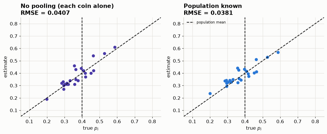

🔑 The estimates got biased, and that is why they got better

Look at the right panel against the dashed identity line. The points are pulled toward the population mean — coins above it are estimated a little low, coins below it a little high. Each individual estimate is now biased.

And yet the RMSE is lower. That is the bias–variance trade in its cleanest form: 100 flips leave real uncertainty about each coin, and borrowing the population’s opinion removes more variance than the bias it adds.

The trade is not free. If a coin genuinely sat far outside the population, this would drag it wrongly, and no amount of pooling would tell you that had happened. Shrinkage is an assumption about how the world is organised, not a free improvement — and it is worth being explicit that you have made it.

4. But we cheated

Method 1 used TRUE_ALPHA and TRUE_BETA — the values that generated the data. In any real study nobody hands you those. So what happens if you guess the population wrong?

guesses = [("true", TRUE_ALPHA, TRUE_BETA),
           ("too tight, wrong centre", 40.0, 10.0),
           ("nearly flat", 1.2, 1.2)]

fig, axes = plt.subplots(1, 3, figsize=(13, 4.0))
for ax, (label, a, b) in zip(axes, guesses):
    ch, _ = metropolis_known_pop(a, b, seed=RANDOM_SEED + 1)
    est = ch[WARMUP:].mean(axis=0)
    r = recovery_panel(ax, est, f"{label}\nBeta({a:g}, {b:g})", S.PRIMARY)
    print(f"  {label:24s} Beta({a:g}, {b:g})  RMSE {r:.4f}")
fig.suptitle("Assuming a population you do not actually know", y=1.02)
fig.tight_layout()

  true                     Beta(10, 15)  RMSE 0.0379
  too tight, wrong centre  Beta(40, 10)  RMSE 0.1526
  nearly flat              Beta(1.2, 1.2)  RMSE 0.0408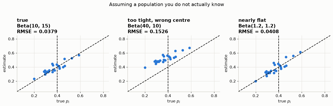

A confidently wrong population is worse than no pooling: it drags every coin toward the wrong place. A nearly flat one is harmless and pointless — it just reproduces the no-pooling answer, since a prior that says nothing lends nothing.

So: we want the pooling, but we do not know where to pool toward. Estimate that too.

5. Method 2 — the hierarchy: estimate \(\alpha\) and \(\beta\) as well

This is the graphical model from the slides. The double-circled nodes are constants we choose; everything else is inferred:

\[ \alpha \sim \text{Gamma}(20, 1), \qquad \beta \sim \text{Gamma}(20, 1), \] \[ p_i \mid \alpha, \beta \sim \text{Beta}(\alpha, \beta), \qquad D_i \mid p_i \sim \text{Bernoulli}(p_i). \]

The sampler alternates two moves: update every \(p_i\) given the current \(\alpha, \beta\), then update \(\alpha, \beta\) given the current \(p_i\). That is Metropolis-within-Gibbs, and it is the whole algorithm.

PRIOR_ALPHA = (20.0, 1.0)      # (shape, rate) for alpha
PRIOR_BETA = (20.0, 1.0)       # (shape, rate) for beta


def log_hyper(alpha, beta, ps):
    """log p(alpha, beta | ps): the Beta density of every coin, times the priors."""
    if alpha <= 0 or beta <= 0:
        return -np.inf
    lp = (stats.gamma.logpdf(alpha, PRIOR_ALPHA[0], scale=1 / PRIOR_ALPHA[1])
          + stats.gamma.logpdf(beta, PRIOR_BETA[0], scale=1 / PRIOR_BETA[1]))
    out = float(np.sum(stats.beta.logpdf(ps, alpha, beta)) + lp)
    return -np.inf if np.isnan(out) else out


def metropolis_hierarchical(n_iter=10_000, tune=0.05, tune_hyper=1.0,
                            seed=RANDOM_SEED):
    """Metropolis-within-Gibbs: the p's, then the hyperparameters, alternating."""
    rng_m = np.random.default_rng(seed)
    p_chain = np.empty((n_iter, S_COINS))
    phi = np.empty((n_iter, 2))                      # columns: alpha, beta

    p_chain[0] = rng_m.beta(1.0, 1.0, S_COINS)
    phi[0] = (5.0, 5.0)
    # Initialise the stored log-density with the SAME target the loop compares
    # against — the R script seeds it with the likelihood alone, which makes the
    # very first accept/reject inconsistent. It self-corrects, but there is no
    # reason to reproduce it.
    lp = np.array([log_post(p_chain[0, j], data[j], *phi[0]) for j in range(S_COINS)])

    n_acc_p, n_acc_h = np.zeros(S_COINS), 0
    for t in range(1, n_iter):
        a_prev, b_prev = phi[t - 1]

        # --- move 1: every coin's p, given the current population -----------
        prop = rng_m.normal(p_chain[t - 1], tune)
        for j in range(S_COINS):
            lp_prop = log_post(prop[j], data[j], a_prev, b_prev)
            if np.log(rng_m.uniform()) < lp_prop - lp[j]:
                p_chain[t, j], lp[j], n_acc_p[j] = prop[j], lp_prop, n_acc_p[j] + 1
            else:
                p_chain[t, j] = p_chain[t - 1, j]

        # --- move 2: the population, given the coins we just updated --------
        a_star, b_star = rng_m.normal(phi[t - 1], tune_hyper)
        num = log_hyper(a_star, b_star, p_chain[t])
        den = log_hyper(a_prev, b_prev, p_chain[t])
        if np.log(rng_m.uniform()) < num - den:
            phi[t], n_acc_h = (a_star, b_star), n_acc_h + 1
        else:
            phi[t] = phi[t - 1]

        # the p-densities were computed under the OLD population; refresh them
        # so the next iteration compares like with like
        if not np.array_equal(phi[t], phi[t - 1]):
            for j in range(S_COINS):
                lp[j] = log_post(p_chain[t, j], data[j], *phi[t])

    return p_chain, phi, n_acc_p / (n_iter - 1), n_acc_h / (n_iter - 1)


p_hier, phi_hier, acc_p, acc_h = metropolis_hierarchical()
print(f"acceptance, coins          : {acc_p.mean():.2f}")
print(f"acceptance, hyperparameters: {acc_h:.2f}")

acceptance, coins          : 0.65
acceptance, hyperparameters: 0.63

BURN = 2000
phi_post = phi_hier[BURN:]
p_post = p_hier[BURN:]

fig, axes = plt.subplots(2, 2, figsize=(11, 6.0))
for k, (name, truth, prior) in enumerate([(r"$\alpha$", TRUE_ALPHA, PRIOR_ALPHA),
                                          (r"$\beta$", TRUE_BETA, PRIOR_BETA)]):
    ax = axes[0, k]
    ax.plot(phi_hier[:, k], lw=0.5, color=S.PRIMARY)
    S.truth_line(ax, truth, label="truth")
    ax.set(title=f"{name} — trace", xlabel="iteration", ylim=(0, 40))
    if k == 0:
        ax.legend(fontsize=8)

    ax = axes[1, k]
    ax.hist(phi_post[:, k], bins=40, density=True, color=S.PRIMARY, alpha=0.75,
            label="posterior")
    g = np.linspace(0, 40, 300)
    ax.plot(g, stats.gamma.pdf(g, prior[0], scale=1 / prior[1]), color=S.ALT,
            lw=2, label="prior")
    S.truth_line(ax, truth, axis="x")
    ax.set(xlabel=name, ylabel="density", xlim=(0, 40))
    ax.legend(fontsize=8)
fig.suptitle("The population parameters, estimated from the coins", y=1.01)
fig.tight_layout()

print(f"alpha: true {TRUE_ALPHA:5.1f}   posterior mean {phi_post[:, 0].mean():5.1f}"
      f"   89% [{np.percentile(phi_post[:, 0], 5.5):.1f}, "
      f"{np.percentile(phi_post[:, 0], 94.5):.1f}]")
print(f"beta : true {TRUE_BETA:5.1f}   posterior mean {phi_post[:, 1].mean():5.1f}"
      f"   89% [{np.percentile(phi_post[:, 1], 5.5):.1f}, "
      f"{np.percentile(phi_post[:, 1], 94.5):.1f}]")

alpha: true  10.0   posterior mean  15.2   89% [11.6, 19.1]
beta : true  15.0   posterior mean  24.5   89% [18.5, 30.9]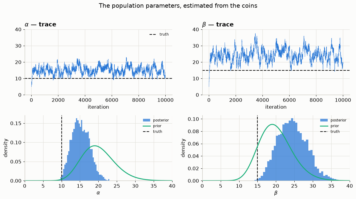

Look at those two panels before moving on. They do not say what a recovery plot usually says: \(\alpha\) sits well above the true 10, \(\beta\) above the true 15, and neither 89% interval covers its truth.

Nothing is broken. Two things are going on.

⚠️ Read the ratio, not the two parameters

\(\alpha\) and \(\beta\) are individually poorly determined and strongly correlated — the plot immediately below shows it. What 24 coins pin down is the population mean \(\alpha/(\alpha+\beta)\). What they say much less about is the total \(\alpha + \beta\), which sets how concentrated the population is, and which is the direction the two parameters trade off along.

So the marginals miss while the quantity the data determined is fine. This is the marginal-versus-joint problem from Day 2 at 15:00, in a model small enough to see whole.

mean_draws = phi_post[:, 0] / (phi_post[:, 0] + phi_post[:, 1])
conc_draws = phi_post[:, 0] + phi_post[:, 1]

fig, (ax1, ax2) = plt.subplots(1, 2, figsize=(11, 4.2))
ax1.plot(phi_post[:, 0], phi_post[:, 1], "o", color=S.PRIMARY, ms=2, alpha=0.1,
         ls="none")
S.truth_point(ax1, TRUE_ALPHA, TRUE_BETA)
r = np.corrcoef(phi_post[:, 0], phi_post[:, 1])[0, 1]
ax1.set(title=rf"joint: corr($\alpha$, $\beta$) = {r:+.2f}", xlabel=r"$\alpha$",
        ylabel=r"$\beta$")
ax1.legend(fontsize=8)

for vals, truth, lbl, colour in [(mean_draws, pop_mean, "mean", S.PRIMARY),
                                 (conc_draws / 100, (TRUE_ALPHA + TRUE_BETA) / 100,
                                  r"total / 100", S.NAIVE)]:
    ax2.hist(vals, bins=40, density=True, color=colour, alpha=0.6, label=lbl)
    ax2.axvline(truth, color=S.TRUTH, ls="--", lw=1.5)
ax2.set(title="what the data actually determined", xlabel="value", ylabel="density")
ax2.legend(fontsize=9)
fig.tight_layout()

cv = lambda v: v.std() / v.mean()
print(f"coefficient of variation — population mean : {cv(mean_draws):.3f}")
print(f"                          total (a + b)    : {cv(conc_draws):.3f}"
      f"   ({cv(conc_draws) / cv(mean_draws):.0f}x less well determined)")

coefficient of variation — population mean : 0.048
                          total (a + b)    : 0.155   (3x less well determined)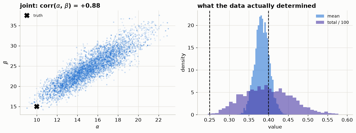

And the prior is doing the rest

The other half of the explanation is the \(\text{Gamma}(20, 1)\) prior. Its mean is 20 — above both true values — so it pushes the concentration up. The R script offers a noninformative alternative on the next line, commented out. Run both and the question settles itself.

def fit_with_prior(pa, pb, label):
    with pm.Model(coords={"coin": np.arange(S_COINS)}):
        a = pm.Gamma("alpha", alpha=pa[0], beta=pa[1])
        b = pm.Gamma("beta", alpha=pb[0], beta=pb[1])
        pp = pm.Beta("p", alpha=a, beta=b, dims="coin")
        pm.Binomial("x", n=N_FLIPS, p=pp, observed=x, dims="coin")
        idt = pm.sample(draws=1500, tune=1500, chains=4, cores=4,
                        nuts_sampler="pymc", target_accept=0.9,
                        progressbar=False, random_seed=RANDOM_SEED)
    d = idt.posterior.dataset
    al, be = d["alpha"].values.ravel(), d["beta"].values.ravel()
    ci = lambda v: np.percentile(v, [5.5, 94.5])
    covers = lambda v, t: "yes" if ci(v)[0] <= t <= ci(v)[1] else "NO"
    print(f"{label}")
    for nm, v, t in [("alpha", al, TRUE_ALPHA), ("beta", be, TRUE_BETA),
                     ("pop. mean", al / (al + be), pop_mean)]:
        lo, hi = ci(v)
        print(f"   {nm:10s} {v.mean():6.2f}   89% [{lo:5.2f}, {hi:6.2f}]"
              f"   covers truth? {covers(v, t)}")
    return idt


_ = fit_with_prior((20.0, 1.0), (20.0, 1.0), "Gamma(20, 1) — 'somewhat informed'")
print()
_ = fit_with_prior((0.1, 0.1), (0.1, 0.1), "Gamma(0.1, 0.1) — noninformative")

Initializing NUTS using jitter+adapt_diag...
Multiprocess sampling (4 chains in 4 jobs)
NUTS: [alpha, beta, p]
Sampling 4 chains for 1_500 tune and 1_500 draw iterations (6_000 + 6_000 draws total) took 1 seconds.
Initializing NUTS using jitter+adapt_diag...
Multiprocess sampling (4 chains in 4 jobs)
NUTS: [alpha, beta, p]

Gamma(20, 1) — 'somewhat informed'
   alpha       15.00   89% [11.54,  18.80]   covers truth? NO
   beta        24.08   89% [18.51,  30.35]   covers truth? NO
   pop. mean    0.38   89% [ 0.36,   0.41]   covers truth? yes

Sampling 4 chains for 1_500 tune and 1_500 draw iterations (6_000 + 6_000 draws total) took 1 seconds.

Gamma(0.1, 0.1) — noninformative
   alpha        9.36   89% [ 5.16,  14.86]   covers truth? yes
   beta        15.36   89% [ 8.41,  24.58]   covers truth? yes
   pop. mean    0.38   89% [ 0.34,   0.42]   covers truth? yes

With the vague prior, \(\alpha\) and \(\beta\) both recover. With the informative one they do not — while the population mean covers the truth either way.

A hyperprior is not a formality you fill in to make the model run. With 24 groups there is little information about the population’s spread, so what you assert about it largely survives into the answer. The \(p_i\) barely notice — they depend on the mean, which the data do determine — but a sentence about \(\alpha\) itself is mostly a sentence about your prior.

Did estimating the population cost us anything?

est_hier = p_post.mean(axis=0)

fig, axes = plt.subplots(1, 3, figsize=(13, 4.2))
r_naive = recovery_panel(axes[0], naive, "No pooling", S.NAIVE)
r_known = recovery_panel(axes[1], est_known, "Population known (cheating)", S.ALT)
r_hier = recovery_panel(axes[2], est_hier, "Hierarchical (estimated)", S.PRIMARY)
axes[2].legend(fontsize=8, loc="upper left")
fig.suptitle("Three answers to the same question", y=1.02)
fig.tight_layout()

print(f"RMSE  no pooling                 {r_naive:.4f}")
print(f"RMSE  population known (cheating){r_known:9.4f}")
print(f"RMSE  hierarchical (estimated)   {r_hier:9.4f}")

RMSE  no pooling                 0.0407
RMSE  population known (cheating)   0.0381
RMSE  hierarchical (estimated)      0.0377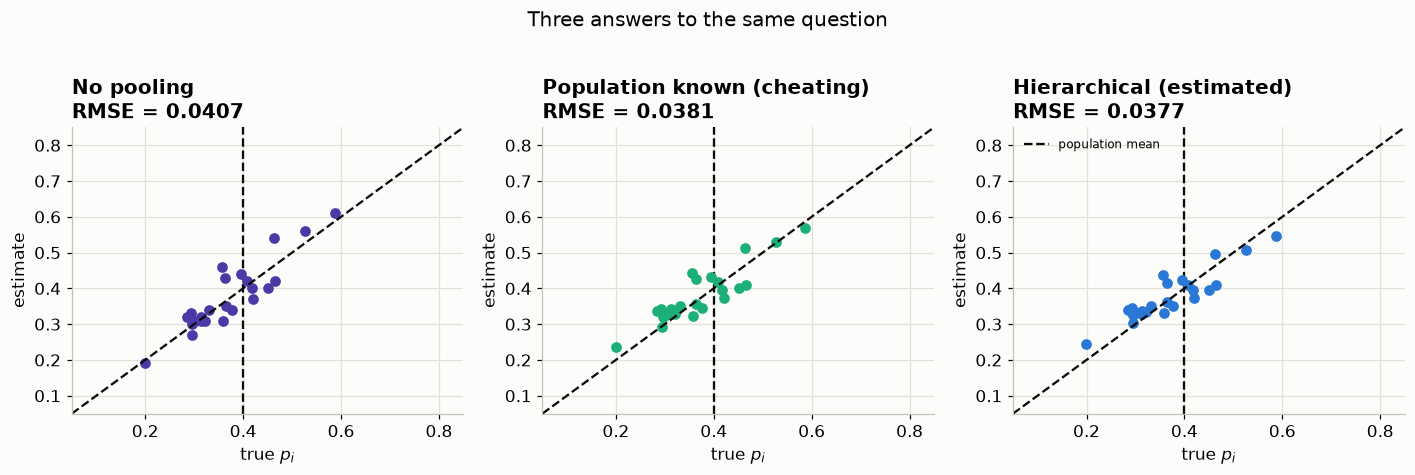

💡 The result worth remembering

The hierarchical fit lands close to the one that was told the right answer, while estimating the population from the same 24 coins it is shrinking. You do not pay much for the honesty.

It works because the population is estimated from all the coins. Each one is noisy, but \(\alpha\) and \(\beta\) see 24 at once, and there is far more information about where coins sit in general than about where coin 7 sits.

Shrinkage, drawn directly

order = np.argsort(true_p)
fig, ax = plt.subplots(figsize=(9.5, 4.2))
for k, j in enumerate(order):
    ax.plot([k, k], [naive[j], est_hier[j]], "-", color=S.MUTED, lw=1, zorder=1)
ax.plot(range(S_COINS), naive[order], "o", color=S.NAIVE, ms=6, ls="none",
        label="no pooling")
ax.plot(range(S_COINS), est_hier[order], "o", color=S.PRIMARY, ms=6, ls="none",
        label="hierarchical")
ax.plot(range(S_COINS), true_p[order], "_", color=S.TRUTH, ms=14, mew=2,
        ls="none", label="truth")
S.truth_line(ax, pop_mean, label="population mean")
ax.set(title="Every coin is pulled toward the population mean",
       xlabel="coin (sorted by true $p$)", ylabel="$p$")
ax.legend(fontsize=9, ncol=2)
fig.tight_layout()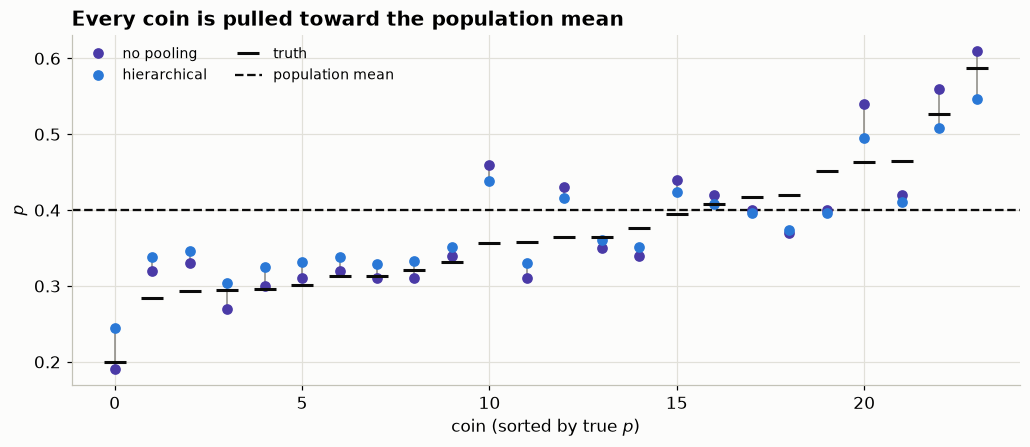

Every arrow points inward, and the outermost coins move furthest. That looks like the model treating extreme coins with extra suspicion. It is not — and the actual rule is simple enough to write down.

Hold \(\alpha, \beta\) fixed for a moment. The Beta is conjugate to the Binomial, so coin \(j\)’s posterior is \(\text{Beta}(\alpha + x_j,\ \beta + n - x_j)\), with mean

\[ \mathbb{E}[p_j] \;=\; \frac{\alpha + x_j}{\alpha + \beta + n} \;=\; \underbrace{w}_{\text{own data}} \cdot \frac{x_j}{n} \;+\; (1 - w) \cdot \underbrace{\frac{\alpha}{\alpha+\beta}}_{\text{population mean}}, \qquad w = \frac{n}{n + \alpha + \beta}. \]

A weighted average, and the weight depends on \(n\) and \(\alpha + \beta\) — not on \(x_j\). So every coin is shrunk by the same fraction; what differs is how far each one has to travel.

a_hat, b_hat = phi_post[:, 0].mean(), phi_post[:, 1].mean()
w = N_FLIPS / (N_FLIPS + a_hat + b_hat)

print(f"alpha + beta = {a_hat + b_hat:5.1f}   <- a 'prior sample size', in flips")
print(f"n            = {N_FLIPS}")
print(f"w            = {w:.3f}    weight on the coin's own flips")
print(f"1 - w        = {1 - w:.3f}    shrinkage, the SAME for all {S_COINS} coins\n")

predicted = w * naive + (1 - w) * (a_hat / (a_hat + b_hat))
print(f"largest gap between that formula and the sampler: "
      f"{np.abs(predicted - est_hier).max():.4f}")

pull = np.abs(naive - est_hier)
far = np.abs(naive - pop_mean) > np.median(np.abs(naive - pop_mean))
print(f"\nabsolute pull  far from the mean : {pull[far].mean():.4f}")
print(f"               near the mean     : {pull[~far].mean():.4f}")
# Pooled ratio, not a mean of per-coin ratios: one coin sits essentially ON the
# population mean, and dividing by its ~zero distance would blow up.
dist = np.abs(naive - pop_mean)
print(f"pull / distance, far             : {pull[far].sum() / dist[far].sum():.3f}")
print(f"                 near            : {pull[~far].sum() / dist[~far].sum():.3f}"
      f"   <- the same fraction")

alpha + beta =  39.6   <- a 'prior sample size', in flips
n            = 100
w            = 0.716    weight on the coin's own flips
1 - w        = 0.284    shrinkage, the SAME for all 24 coins

largest gap between that formula and the sampler: 0.0023

absolute pull  far from the mean : 0.0328
               near the mean     : 0.0113
pull / distance, far             : 0.268
                 near            : 0.308   <- the same fraction

The last two numbers are the point. In absolute terms the extreme coins move about three times as far; as a fraction of their distance to the population mean, every coin moves by the same amount. Nothing is treating extreme coins specially — they simply start further away.

🔑 What actually controls how much a group shrinks

Read \(\alpha + \beta\) as a prior sample size, measured in flips. Here it is about 40, against \(n = 100\) real flips per coin, so each coin’s estimate is roughly 70% its own data and 30% the population. Change either number and the weight moves:

flips per coin	\(1 - w\), the shrinkage
10	0.80
100	0.28
1000	0.04

Data quantity is the knob. A group with few observations is shrunk hard; a group with many is left alone. Every coin here has exactly 100 flips, which is why the fraction came out constant and only the distance varied — that is a property of this tidy simulated design, not of hierarchical models.

In hierarchical-mcmc.ipynb the participants deliberately differ in how much data they contribute, and you will see the same formula produce different shrinkage per participant. Same rule, different thing varying.

6. The same model, in PyMC

Everything above was written out so that nothing is mysterious. Here is the identical model as PyMC states it — and note that we can use the number of heads rather than the individual flips, since a Binomial count is a sufficient statistic for a sequence of Bernoulli trials.

with pm.Model(coords={"coin": np.arange(S_COINS)}) as hier_model:
    alpha = pm.Gamma("alpha", alpha=PRIOR_ALPHA[0], beta=PRIOR_ALPHA[1])
    beta = pm.Gamma("beta", alpha=PRIOR_BETA[0], beta=PRIOR_BETA[1])
    p = pm.Beta("p", alpha=alpha, beta=beta, dims="coin")
    pm.Binomial("x", n=N_FLIPS, p=p, observed=x, dims="coin")

pm.model_to_graphviz(hier_model)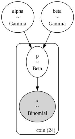

That graph is the slide’s diagram, drawn by the library from the model you wrote. The box is the plate over coins; alpha and beta sit outside it, shared.

with hier_model:
    idata = pm.sample(draws=1500, tune=1500, chains=4, cores=4,
                      nuts_sampler="pymc", target_accept=0.9,
                      progressbar=False, random_seed=RANDOM_SEED)

print(az.summary(idata, var_names=["alpha", "beta"], kind="all").to_string())
print(f"\ntruth: alpha = {TRUE_ALPHA}, beta = {TRUE_BETA}")

Initializing NUTS using jitter+adapt_diag...
Multiprocess sampling (4 chains in 4 jobs)
NUTS: [alpha, beta, p]
Sampling 4 chains for 1_500 tune and 1_500 draw iterations (6_000 + 6_000 draws total) took 1 seconds.

        mean    sd eti89_lb eti89_ub  ess_bulk  ess_tail r_hat mcse_mean mcse_sd
alpha     15  2.27       12       19      8220      4900  1.00     0.025   0.018
beta   24.08  3.67       19       30      8335      5072  1.00      0.04   0.029

truth: alpha = 10.0, beta = 15.0

Does the thirty-line sampler agree with the library?

post = idata.posterior.dataset
pymc_alpha = post["alpha"].values.ravel()
pymc_beta = post["beta"].values.ravel()
est_pymc = post["p"].values.reshape(-1, S_COINS).mean(axis=0)

fig, (ax1, ax2) = plt.subplots(1, 2, figsize=(11, 4.2))
for vals, colour, lbl in [(phi_post[:, 0], S.NAIVE, "hand-written"),
                          (pymc_alpha, S.PRIMARY, "PyMC / NUTS")]:
    ax1.hist(vals, bins=40, density=True, color=colour, alpha=0.55, label=lbl)
S.truth_line(ax1, TRUE_ALPHA, axis="x")
ax1.set(title=r"posterior for $\alpha$", xlabel=r"$\alpha$", ylabel="density")
ax1.legend(fontsize=9)

ax2.plot(est_hier, est_pymc, "o", color=S.PRIMARY, ms=6, ls="none")
lims = (0.05, 0.85)
ax2.plot(lims, lims, "--", color=S.TRUTH, lw=1.5)
ax2.set(title="per-coin estimates agree", xlabel="hand-written sampler",
        ylabel="PyMC", xlim=lims, ylim=lims)
fig.tight_layout()

print(f"alpha  hand-written {phi_post[:, 0].mean():5.2f}   PyMC {pymc_alpha.mean():5.2f}")
print(f"beta   hand-written {phi_post[:, 1].mean():5.2f}   PyMC {pymc_beta.mean():5.2f}")
print(f"largest per-coin disagreement: {np.abs(est_hier - est_pymc).max():.4f}")

alpha  hand-written 15.19   PyMC 15.00
beta   hand-written 24.46   PyMC 24.08
largest per-coin disagreement: 0.0021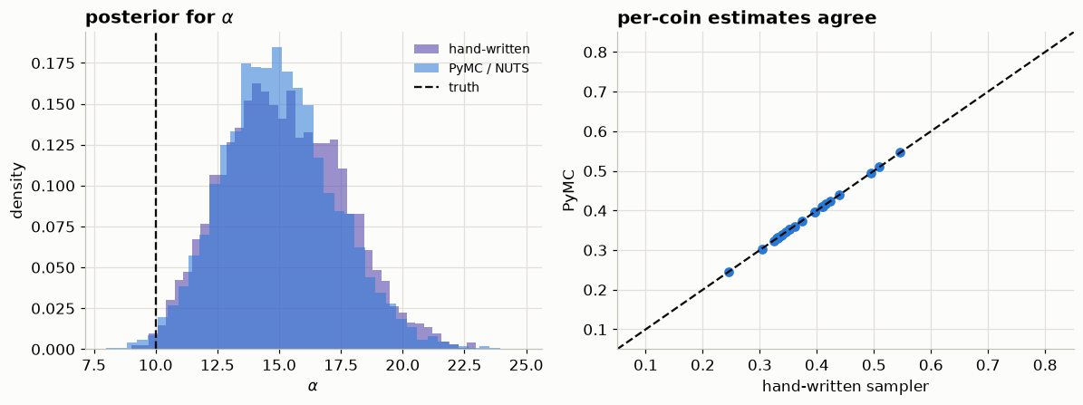

They agree, which is the point of writing the sampler out: PyMC is doing the same thing, faster and with better diagnostics.

Worth quantifying “faster”. Ours ran 10,000 iterations; NUTS ran 1,500 draws per chain and returns a far larger effective sample size, because a random walk in 26 dimensions — 24 coins plus two hyperparameters — is a poor way to explore.

ess_pymc = float(az.ess(idata, var_names=["alpha"]).alpha)
dt_hand = az.convert_to_datatree({"alpha": phi_post[None, :, 0]})
ess_hand = float(az.ess(dt_hand, var_names=["alpha"]).alpha)
print(f"ESS for alpha — hand-written: {ess_hand:7.1f} out of {phi_post.shape[0]:,} draws")
print(f"                PyMC / NUTS : {ess_pymc:7.1f} out of "
      f"{post.sizes['chain'] * post.sizes['draw']:,} draws")

ESS for alpha — hand-written:    65.7 out of 8,000 draws
                PyMC / NUTS :  8220.4 out of 6,000 draws

7. Exercises

Exercise 1 — how many coins do you need?

The population was estimated from 24 coins. Re-run the PyMC model with the first 5 coins only, and compare the width of the posterior for the population mean. How much of the hierarchy’s benefit survives?

Solution

k = 5
with pm.Model(coords={"coin": np.arange(k)}) as small:
    a = pm.Gamma("alpha", alpha=PRIOR_ALPHA[0], beta=PRIOR_ALPHA[1])
    b = pm.Gamma("beta", alpha=PRIOR_BETA[0], beta=PRIOR_BETA[1])
    pp = pm.Beta("p", alpha=a, beta=b, dims="coin")
    pm.Binomial("x", n=N_FLIPS, p=pp, observed=x[:k], dims="coin")
    idata_small = pm.sample(draws=1500, tune=1500, chains=4, cores=4,
                            nuts_sampler="pymc", target_accept=0.9,
                            progressbar=False, random_seed=RANDOM_SEED)

With five coins the population is barely identified and the posterior for \(\alpha\) leans heavily on its Gamma prior. The shrinkage still happens, but it is being driven by your prior rather than by the data — which is fine as long as you know it, and misleading if you do not.

Exercise 2 — an outlier coin

Set true_p[0] = 0.95 before generating the data, so one coin genuinely does not belong to the population. Refit. What happens to that coin’s estimate, and to \(\alpha\) and \(\beta\)?

What to notice

Two things, and the second is the one people miss. The outlier is pulled sharply downward — the model does not believe it. And the population is dragged toward it, so every other coin’s estimate moves too.

That is the cost of the assumption stated plainly: in a hierarchical model there is no such thing as a local error. A single badly-behaved participant contaminates the group parameters, and through them everyone else. Fixes exist — a heavier-tailed population, or an explicit mixture with an outlier component — and all of them amount to saying out loud what you think the population really looks like.

What to take away

💡 The four things that matter

1. A hierarchy is a prior you estimate. The population distribution is a prior on each coin, and the only new idea is that its parameters are unknown and inferred alongside everything else.
2. Shrinkage is deliberate bias that lowers error. Individual estimates move toward the population mean, and the extreme ones move most. Here that cut RMSE against no pooling at all.
3. Estimating the population costs surprisingly little. The hierarchical fit came close to the one handed the true \(\alpha, \beta\) — because the population is informed by every coin at once.
4. Read the joint. \(\alpha\) and \(\beta\) are individually poorly determined and strongly correlated; the population mean is what the data pin down. Reporting a marginal interval for \(\alpha\) alone would misstate the result — here those intervals miss the truth while the mean covers it.
5. The hyperprior is a real assumption. With 24 groups there is little information about the population’s spread, so what you assert about it survives into the answer. Swapping Gamma(20, 1) for Gamma(0.1, 0.1) moved \(\alpha\) from 15.0 to 9.4 against a truth of 10.

Where this goes next. hierarchical-mcmc.ipynb picks up exactly here and asks what this model does to the geometry of the posterior — the funnel that appears when a group-level scale gets small, why it biases the answer rather than merely slowing the sampler, and what centered versus non-centered parameterization does about it.