Simulating data from a cognitive model

Day 2, 14:00 — 30 minutes. Alexander Fengler.

A cognitive model is, first and last, a generative story: parameters in, data out. Before you fit anything, you should be able to push parameters through the model and look at what comes back. That is what this session is about.

We use ssm-simulators, the simulation layer of the HSSM ecosystem. It ships fast compiled simulators for a large family of sequential-sampling models, and it is what generates the training data behind the neural likelihoods you will meet tomorrow.

By the end you will have:

1. simulated from a model and understood the shape rules,
2. discovered the model zoo by introspection rather than by memorising names,
3. built your own model and simulated from it,
4. produced the dataset we dissect in the next session.

▶️ Running this on Google Colab

The cell below is a no-op on your own machine. On Colab it installs the stack and downloads the shared helper module, which lives one directory up in the repository and is therefore not importable there.

Expect the install to take a few minutes. If Colab asks you to restart the runtime, do it and then run the cell again — the second run is a no-op.

# --- Google Colab bootstrap; does nothing anywhere else ---------------------
import importlib.util, subprocess, sys, urllib.error, urllib.request

IN_COLAB = importlib.util.find_spec("google.colab") is not None

# `main` once this is merged; the branch is the fallback so the Colab path can
# be tested BEFORE the merge, when main does not yet have these files.
_REFS = ("main", "afengler.tutorials")
_RAW = "https://raw.githubusercontent.com/stefanradev93/sbi4cogsci/{ref}/tutorials/"


def _fetch(module):
    for ref in _REFS:
        try:
            urllib.request.urlretrieve(_RAW.format(ref=ref) + module, module)
            return ref
        except urllib.error.HTTPError:
            continue
    raise RuntimeError(f"could not fetch {module} from any of {_REFS}")


if IN_COLAB:
    subprocess.run([sys.executable, "-m", "pip", "install", "-q", "ssm-simulators>=0.13.2", "matplotlib"],
                   check=True)
    for _mod in ["sbi4cogsci_style.py"]:
        print(f"  fetched {_mod} from {_fetch(_mod)}")
    print("Colab setup done.")

import sys, pathlib, warnings
sys.path.insert(0, str(pathlib.Path.cwd().parent))  # -> tutorials/

import numpy as np
import matplotlib.pyplot as plt
import sbi4cogsci_style as S

S.use()
warnings.filterwarnings("ignore", category=UserWarning)

import ssms
from ssms import Simulator
from ssms.config import model_config

RANDOM_SEED = sum(map(ord, "sbi4cogsci-simulate"))
rng = np.random.default_rng(RANDOM_SEED)

print("ssm-simulators", ssms.__version__ if hasattr(ssms, "__version__") else "0.13.2")

ssm-simulators 0.13.2

1. One call, and the shape rules

The drift-diffusion model has four parameters: drift v, boundary height a, relative start point z, and non-decision time t. Here the process runs between \(+a\) and \(-a\), so a is the distance from zero to one bound — you will also see “boundary separation” used for the full gap, which is \(2a\).

The main entry point is the Simulator class. You build one for a model, then call .simulate() as often as you like — the model configuration is resolved once, at construction, rather than on every call.

sim = Simulator(model="ddm")

out = sim.simulate(theta=[0.5, 1.2, 0.5, 0.3],
                   n_samples=500,
                   random_state=RANDOM_SEED,
                   )

print("returned keys:", sorted(out.keys()))
print("rts    ", out["rts"].shape)
print("choices", out["choices"].shape, "->", np.unique(out["choices"]))

returned keys: ['choices', 'metadata', 'rts']
rts     (500, 1)
choices (500, 1) -> [-1  1]

Three things to notice, all of which cost people time:

1. Choices are coded -1 and +1, not 0/1. This convention runs through the whole ecosystem — HSSM will reject other codings for 2-choice models, and a valid-but-wrong 0/1 coding silently mismodels bias.
2. The response key is choices, and rts is 2-D — (n_samples, 1), not a flat vector.

The shape rule

There are three ways to ask for data, and mixing them up is the single most common error. What you get back depends on both how many parameter sets you hand in and how many samples you ask for:

You want	theta	n_samples	shape of rts
many trials, one parameter set	vector (n_params,)	n	(n, 1)
one trial each, many parameter sets	matrix (n_trials, n_params)	1	(n_trials, 1)
many samples per parameter set	matrix (n_trials, n_params)	n	(n, n_trials, 1)

The second form is how trial-varying parameters work — one row per trial — and is what you need when drift depends on a condition, a covariate, or a stimulus. The third is what you want for a parameter sweep, where you need a whole distribution at each setting rather than a single draw.

# Third form: 7 parameter settings, 20 samples each.
theta_sweep = np.column_stack([
    np.linspace(-2.0, 2.0, 7),   # v varies
    np.full(7, 1.2),             # a
    np.full(7, 0.5),             # z
    np.full(7, 0.3),             # t
])
swept = sim.simulate(theta=theta_sweep, n_samples=20, random_state=RANDOM_SEED)
print("theta", theta_sweep.shape, "with n_samples=20 ->",
      "rts", swept["rts"].shape, "  (n_samples, n_trials, 1)")

theta (7, 4) with n_samples=20 -> rts (20, 7, 1)   (n_samples, n_trials, 1)

Now the trial-varying form, at a scale that also tells us something about speed: 100,000 trials, drift ramping from strongly negative to strongly positive.

n_trials = 100_000
V_LO, V_HI = -5.0, 5.0
v_by_trial = np.linspace(V_LO, V_HI, n_trials)
theta_matrix = np.column_stack([
    v_by_trial,
    np.full(n_trials, 1.2),   # a
    np.full(n_trials, 0.5),   # z
    np.full(n_trials, 0.3),   # t
])

trialwise = sim.simulate(theta=theta_matrix, n_samples=1, random_state=RANDOM_SEED)
rt = trialwise["rts"].flatten()
ch = trialwise["choices"].flatten()

fig, (ax1, ax2) = plt.subplots(1, 2, figsize=(11, 3.6))
ax1.plot(v_by_trial, rt, "o", color=S.PRIMARY, ms=1, alpha=0.10, ls="none")
ax1.set(title="Drift controls speed", xlabel="drift $v$", ylabel="RT (s)",
        ylim=(0, 4))

# Choice proportion in drift bins — binned across the FULL simulated range.
bins = np.linspace(V_LO, V_HI, 41)
idx = np.digitize(v_by_trial, bins) - 1
prop = [np.mean(ch[idx == i] == 1) if (idx == i).sum() else np.nan
        for i in range(len(bins) - 1)]
ax2.plot(0.5 * (bins[:-1] + bins[1:]), prop, "-", color=S.PRIMARY, lw=2,
         label="simulated")
S.truth_line(ax2, 0.5, label="chance")
ax2.set(title="...and accuracy", xlabel="drift $v$", ylabel="P(choice = +1)",
        ylim=(0, 1))
ax2.legend()
fig.tight_layout()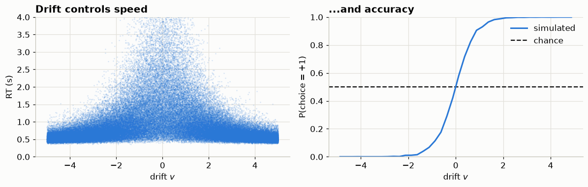

Accuracy saturates: past roughly \(|v| = 3\) every trial goes the same way, and pushing drift higher buys nothing observable. Hold on to that — it is the mechanism behind the identifiability failure in the next session.

2. How fast is this, and does threading help?

You just simulated 100,000 trials. Worth knowing what that cost, because the answer determines whether you ever need to think about performance again.

import time

t0 = time.time()
sim.simulate(theta=theta_matrix, n_samples=1, random_state=RANDOM_SEED)
elapsed = time.time() - t0
print(f"{n_trials:,} trials in {elapsed:.2f}s  "
      f"({n_trials / elapsed / 1000:.0f}k trials/second)")

100,000 trials in 0.82s  (122k trials/second)

The simulators are compiled Cython, so this is fast enough that simulation is rarely your bottleneck — fitting is.

simulate() also takes an n_threads argument. Whether it does anything depends on how your copy was built, and ssm-simulators ships a diagnostic that tells you:

from cssm import _openmp_status

_openmp_status.print_status()

============================================================
SSMS Parallel Execution Status
============================================================
  OpenMP compiled:    Yes
  GSL compiled:       Yes
  Parallel ready:     Yes
  Max threads (OMP):  18
  Max threads limit:  256 (compile-time)
  CPU processors:     18
  OMP_NUM_THREADS:    (not set)
  Python cpu_count:   18
============================================================

📝 If yours says OpenMP compiled: No

The prebuilt wheels on PyPI are compiled without OpenMP, so n_threads is accepted and ignored. That is what most people will see, and nothing in this course needs threading.

To turn it on you have to build from source against a local OpenMP. On macOS:

brew install libomp
export LIBOMP=$(brew --prefix libomp)
export CFLAGS="-Xpreprocessor -fopenmp -I$LIBOMP/include"
export LDFLAGS="-L$LIBOMP/lib -lomp"
uv pip install --no-binary ssm-simulators --reinstall-package ssm-simulators \
    "ssm-simulators==0.13.2"

On Linux libgomp usually comes with gcc and plain CFLAGS="-fopenmp" is enough. Note a later uv sync reinstalls the wheel and silently undoes this — re-run the command if n_threads stops helping.

Does threading actually help? Measure it

Only if OpenMP is compiled in — and then only for the right shape of workload. This is the shape rule from section 1 showing up again as a performance question.

if _openmp_status.is_openmp_available():
    def bench(model, theta, n_samples, label):
        sim_b = Simulator(model=model)
        times = []
        for nt in (1, 8):
            sim_b.simulate(theta=theta, n_samples=n_samples, random_state=1,
                           n_threads=nt)                      # warm up
            t0 = time.time()
            sim_b.simulate(theta=theta, n_samples=n_samples, random_state=1,
                           n_threads=nt)
            times.append(time.time() - t0)
        print(f"  {label:38s} 1 thread {times[0]:5.2f}s   "
              f"8 threads {times[1]:5.2f}s   speedup {times[0] / times[1]:4.2f}x")

    n_sweep = 2_000
    theta_many = np.column_stack([np.linspace(-2, 2, n_sweep), np.full(n_sweep, 1.2),
                                  np.full(n_sweep, 0.5), np.full(n_sweep, 0.3)])
    bench("ddm", theta_matrix, 1, "100k trials x 1 sample")
    bench("ddm", theta_many, 200, "2k trials x 200 samples")
else:
    print("OpenMP not compiled in — n_threads is accepted and ignored. "
          "See the note above.")

  100k trials x 1 sample                 1 thread  0.82s   8 threads  0.93s   speedup 0.87x
  2k trials x 200 samples                1 thread  1.88s   8 threads  0.31s   speedup 6.12x

The two rows go in opposite directions, and the reason is worth knowing.

Threading parallelises the samples drawn for each parameter set. The trial-varying shape — 100,000 rows, one sample each — gives every thread a single short random walk, so coordination costs more than the work itself and threading comes out slower than one thread. The sweep shape — a couple of thousand rows with hundreds of samples each — hands every thread a real chunk of work, and it goes several times faster.

The general lesson is the one that applies to every parallelism knob you will ever meet: it is not free, and whether it pays depends on the granularity of the work. Measure on your own workload rather than assuming more threads is better. And note that neither row is a bottleneck at this scale — both are under a couple of seconds for hundreds of thousands of trials.

3. The model zoo, by introspection

Do not memorise the model list — interrogate it. Every model carries its own parameter names and the box those parameters live in.

import textwrap

names = sorted(model_config.keys())
print(f"{len(names)} models registered. The first 30, alphabetically:\n")
print(textwrap.fill(", ".join(names[:30]), width=76,
                    initial_indent="   ", subsequent_indent="   "))
print(f"\n   ... and {len(names) - 30} more.")

113 models registered. The first 30, alphabetically:

   addm, angle, conflict_ds, conflict_ds_angle, conflict_dsstimflex,
   conflict_dsstimflex_angle, conflict_stimflex, conflict_stimflex_angle,
   conflict_stimflexrel1, conflict_stimflexrel1_angle,
   conflict_stimflexrel1_leak, conflict_stimflexrel1_leak2, ddm, ddm_legacy,
   ddm_mic2_adj, ddm_mic2_adj_angle_no_bias,
   ddm_mic2_adj_conflict_gamma_no_bias, ddm_mic2_adj_no_bias,
   ddm_mic2_adj_weibull_no_bias, ddm_mic2_leak, ddm_mic2_leak_angle_no_bias,
   ddm_mic2_leak_angle_no_bias_no_lowdim_noise,
   ddm_mic2_leak_conflict_gamma_no_bias,
   ddm_mic2_leak_conflict_gamma_no_bias_no_lowdim_noise,
   ddm_mic2_leak_no_bias, ddm_mic2_leak_no_bias_no_lowdim_noise,
   ddm_mic2_leak_weibull_no_bias,
   ddm_mic2_leak_weibull_no_bias_no_lowdim_noise,
   ddm_mic2_multinoise_angle_no_bias,
   ddm_mic2_multinoise_conflict_gamma_no_bias

   ... and 83 more.

Each entry is a plain dictionary. Look at one in full — this is the whole contract a model has to satisfy:

cfg = model_config["angle"]
for key, value in cfg.items():
    shown = value if not callable(value) else f"<callable {getattr(value, '__name__', '?')}>"
    print(f"  {key:<22} {str(shown)[:70]}")

  name                   angle
  params                 ['v', 'a', 'z', 't', 'theta']
  param_bounds           [[-3.0, 0.3, 0.1, 0.001, -0.1], [3.0, 3.0, 0.9, 2.0, 1.3]]
  boundary_name          angle
  boundary               <callable angle>
  n_params               5
  default_params         [0.0, 1.0, 0.5, 0.001, 0.0]
  nchoices               2
  choices                [-1, 1]
  n_particles            1
  simulator              <callable ddm_flexbound>
  parameter_transforms   {'sampling': [], 'simulation': []}
  param_bounds_dict      {'v': (-3.0, 3.0), 'a': (0.3, 3.0), 'z': (0.1, 0.9), 't': (0.001, 2.0)

The two fields you will reach for constantly are params (the names, in the order the simulator expects them) and param_bounds (the box they are valid in). Compare a few models:

for name in ["ddm", "angle", "weibull", "lba3"]:
    c = model_config[name]
    lo, hi = c["param_bounds"]
    box = ", ".join(f"{p} [{l:g}, {h:g}]" for p, l, h in zip(c["params"], lo, hi))
    print(f"{name:8s} choices={str(c['choices']):9s} {box}")

ddm      choices=[-1, 1]   v [-3, 3], a [0.3, 2.5], z [0.1, 0.9], t [0, 2]
angle    choices=[-1, 1]   v [-3, 3], a [0.3, 3], z [0.1, 0.9], t [0.001, 2], theta [-0.1, 1.3]
weibull  choices=[-1, 1]   v [-2.5, 2.5], a [0.3, 2.5], z [0.2, 0.8], t [0.001, 2], alpha [0.31, 4.99], beta [0.31, 6.99]
lba3     choices=[0, 1, 2] A [0, 1], b [0, 1], v0 [0, 1], v1 [0.1, 1.1], v2 [0.1, 0.5]

angle is the DDM plus one parameter, theta, which tilts the decision boundary inward over time — the evidence needed to commit decreases the longer you deliberate. Look at what that does, both to the boundary and to the RT distribution.

fig, (ax1, ax2) = plt.subplots(1, 2, figsize=(11.5, 4.0))

# Left: the boundaries. Draw BOTH of them — a two-choice model has an upper and
# a lower bound, the start point sits between them, and evidence terminates at
# whichever it reaches first. Showing only the upper one hides half the model.
t_grid = np.linspace(0, 3, 200)
a0 = 1.5
ax1.plot(t_grid, np.full_like(t_grid, a0), color=S.PRIMARY, lw=2,
         label="ddm (constant)")
ax1.plot(t_grid, -np.full_like(t_grid, a0), color=S.PRIMARY, lw=2)
for theta_val, ls in [(0.4, "--"), (0.8, ":")]:
    bound = np.maximum(a0 - np.tan(theta_val) * t_grid, 0)
    ax1.plot(t_grid, bound, color=S.NAIVE, linestyle=ls, lw=2,
             label=f"angle, $\\theta$={theta_val}")
    ax1.plot(t_grid, -bound, color=S.NAIVE, linestyle=ls, lw=2)
ax1.axhline(0.0, color=S.MUTED, lw=1, ls="-")           # start point, z = 0.5
ax1.text(2.95, 0.06, "start point ($z = 0.5$)", fontsize=8, color=S.MUTED, ha="right")
ax1.text(2.95, a0 * 0.72, "upper: choice $+1$", fontsize=9, color=S.MUTED, ha="right")
ax1.text(2.95, -a0 * 0.72, "lower: choice $-1$", fontsize=9, color=S.MUTED,
         ha="right", va="top")
ax1.set(title="Both decision boundaries over time", xlabel="time (s)",
        ylabel="evidence", ylim=(-1.8, 1.8))
ax1.legend(loc="lower left", fontsize=8)

# Right: what that does to RTs, split by which boundary was reached.
for name, theta, colour in [("ddm", [0.5, 1.5, 0.5, 0.3], S.PRIMARY),
                            ("angle", [0.5, 1.5, 0.5, 0.3, 0.8], S.NAIVE)]:
    o = Simulator(model=name).simulate(theta=theta, n_samples=6000,
                                       random_state=RANDOM_SEED)
    S.signed_rt_hist(ax2, o["rts"], o["choices"], color=colour, label=name)
ax2.set(title="Collapsing bounds shorten the tail", ylabel="density")
S.label_choice_axis(ax2, rt_max=4.0)
ax2.legend(loc="upper left", fontsize=9)
fig.tight_layout()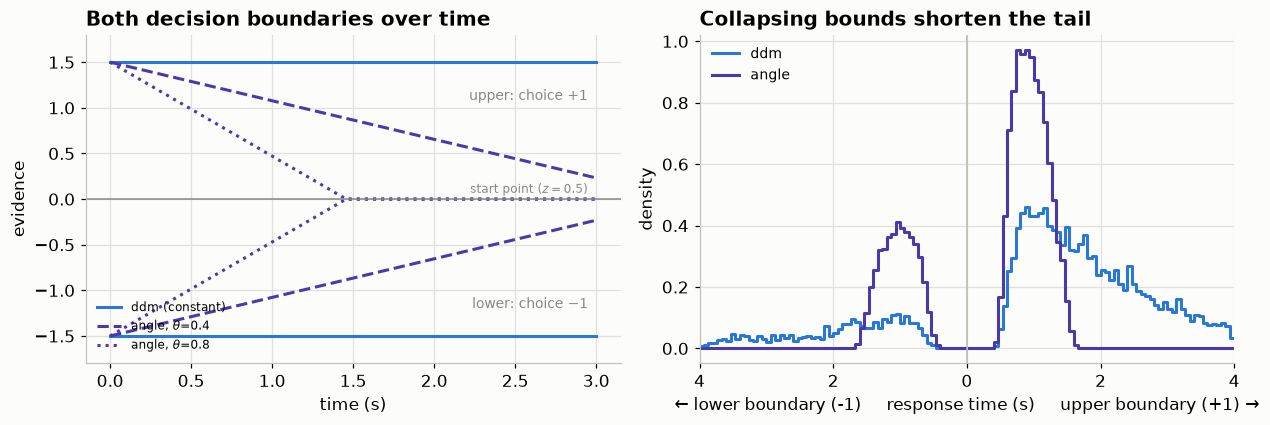

That is the whole game: a parameter with a mechanistic meaning produces a specific, visible signature in the data. Model building is choosing which signatures you want to be able to express.

Turn the knobs yourself

Two tools, both browser-based:

• ssms-gui — a dashboard for playing with ssm-simulators output directly, across the model zoo rather than just the DDM. Built for exactly this kind of build-intuition exploration.
• DDM explorer — a companion page for this session: sliders over drift and boundary separation, showing what each does to the response-time distributions and to accuracy.

Exercise 1

Pick any model from the zoo that we have not plotted, print its parameters and bounds, simulate 2000 trials at a setting of your choice, and plot the RT distribution split by choice.

One solution

name = "weibull"
c = model_config[name]
print(c["params"], c["param_bounds"])

# v, a, z, t, alpha, beta  — alpha/beta shape the collapsing boundary
o = Simulator(model=name).simulate(
    theta=[0.6, 1.4, 0.5, 0.3, 2.0, 2.5], n_samples=2000, random_state=0)
rt, ch = o["rts"].flatten(), o["choices"].flatten()

fig, ax = plt.subplots(figsize=(6, 3.5))
for c_val, colour, lbl in [(1, S.PRIMARY, "+1"), (-1, S.NAIVE, "-1")]:
    ax.hist(rt[ch == c_val], bins=50, range=(0, 4), density=True,
            histtype="step", lw=2, color=colour, label=f"choice {lbl}")
ax.set(xlabel="RT (s)", ylabel="density", title=f"{name}: RT by choice")
ax.legend()

4. Capstone — build your own model

Two routes, depending on how far from a diffusion you want to go. Both are about fifteen lines.

Route A — keep the diffusion machinery, change the boundary

Step 1 — write the function. Nothing library-specific: it takes time t plus its own parameters, and returns the boundary at that time.

import numpy as np
from ssms.config import ModelConfigBuilder


def exp_collapse(t, a=1.0, rate=0.5):
    """Exponentially collapsing boundary: a * exp(-rate * t)."""
    return a * np.exp(-rate * np.asarray(t))


# It is an ordinary function; call and plot it before involving ssms at all.
print("at t=0:", exp_collapse(0.0, a=1.5, rate=0.6),
      " at t=1:", round(float(exp_collapse(1.0, a=1.5, rate=0.6)), 3))

at t=0: 1.5  at t=1: 0.823

Step 2 — describe the model. One call. A model config is the dictionary that fully describes a model — model_config["ddm"] from section 3 was one. from_model copies an existing one and overrides the keys you name, so you inherit everything about the DDM and change only what you mean to.

Four of the overrides swap in the boundary; three declare the new parameter.

cfg_custom = ModelConfigBuilder.from_model(
    "ddm",
    name="ddm_exp_collapse",
    # --- the boundary ---
    boundary=exp_collapse,            # the function itself
    boundary_name="exp_collapse",     # a label, for printing and metadata
    boundary_params=["a", "rate"],    # which parameters it receives
    # --- declare `rate` as a parameter of the model ---
    params=["v", "a", "z", "t", "rate"],
    n_params=5,
    param_bounds=[[-3.0, 0.3, 0.1, 0.0, 0.0],
                  [3.0, 2.5, 0.9, 2.0, 3.0]],
    default_params=[0.0, 1.0, 0.5, 0.001, 0.5],
)

print("params           :", cfg_custom["params"])
print("boundary_params  :", cfg_custom["boundary_params"])
print("param_bounds_dict:", cfg_custom["param_bounds_dict"])

params           : ['v', 'a', 'z', 't', 'rate']
boundary_params  : ['a', 'rate']
param_bounds_dict: {'v': (-3.0, 3.0), 'a': (0.3, 2.5), 'z': (0.1, 0.9), 't': (0.0, 2.0), 'rate': (0.0, 3.0)}

🔑 Why a is in both lists — it is applied once

The two lists answer different questions, which is why a appears in both:

• params — the parameters you pass in theta. This is the model’s public interface: priors, bounds, and the sampling ranges used to train a neural likelihood all read this.
• boundary_params — a routing declaration. Which of those parameters get forwarded to your boundary function.

So a is listed twice but used once: it is a model parameter, and the boundary function is what consumes it. The compiled simulator does not multiply by a again — your function’s return value is the boundary. Every built-in agrees: constant takes ["a"], angle takes ["a", "theta"], weibull_cdf takes ["a", "alpha", "beta"].

You can check this rather than take it on faith — the simulator hands back the boundary it actually used, and we do exactly that two cells below.

Step 3 — simulate from it. From here it is an ordinary model.

my_sim = Simulator(model=cfg_custom)
A0, RATES = 1.5, [0.15, 1.2]
runs = {r: my_sim.simulate(theta={"v": 0.8, "a": A0, "z": 0.5, "t": 0.2, "rate": r},
                           n_samples=6000, random_state=RANDOM_SEED)
        for r in RATES}

# The same two-panel look as the `angle` figure above: the boundary on the left,
# what it does to the data on the right.
fig, (ax1, ax2) = plt.subplots(1, 2, figsize=(11.5, 4.0))

# Left: both bounds, from OUR function — no hard-coded formula, so the picture
# cannot drift away from what was actually simulated.
t_grid = np.linspace(0, 3, 200)
ax1.plot(t_grid, np.full_like(t_grid, A0), color=S.PRIMARY, lw=2,
         label="ddm (constant)")
ax1.plot(t_grid, -np.full_like(t_grid, A0), color=S.PRIMARY, lw=2)
for r, ls in zip(RATES, ["--", ":"]):
    bound = exp_collapse(t_grid, a=A0, rate=r)
    ax1.plot(t_grid, bound, color=S.NAIVE, linestyle=ls, lw=2,
             label=f"exp_collapse, rate={r}")
    ax1.plot(t_grid, -bound, color=S.NAIVE, linestyle=ls, lw=2)
ax1.axhline(0.0, color=S.MUTED, lw=1, ls="-")           # start point, z = 0.5
# Labels sit clear of the exponential, which unlike the linear `angle` bound
# hugs zero on the right-hand side of the panel.
ax1.text(0.06, 0.10, "start point ($z = 0.5$)", fontsize=8, color=S.MUTED)
ax1.text(2.95, 1.74, "upper: choice $+1$", fontsize=9, color=S.MUTED,
         ha="right", va="center")
ax1.text(0.06, -1.74, "lower: choice $-1$", fontsize=9, color=S.MUTED,
         ha="left", va="center")
ax1.set(title="Both decision boundaries over time", xlabel="time (s)",
        ylabel="evidence", ylim=(-1.95, 1.95))
ax1.legend(loc="lower right", fontsize=8)

# Right: what that does to RTs, split by which boundary was reached.
for r, colour, lbl in [(RATES[0], S.PRIMARY, f"rate = {RATES[0]} (slow collapse)"),
                       (RATES[1], S.NAIVE, f"rate = {RATES[1]} (fast collapse)")]:
    o = runs[r]
    lower, upper = S.signed_rt_hist(ax2, o["rts"], o["choices"],
                                    color=colour, label=lbl)
    print(f"{lbl:32s} P(upper) = {upper:.3f}")
ax2.set(title="A boundary you invented, five minutes ago", ylabel="density")
S.label_choice_axis(ax2, rt_max=4.0)
ax2.legend(loc="upper left", fontsize=9)
fig.tight_layout()

rate = 0.15 (slow collapse)      P(upper) = 0.882
rate = 1.2 (fast collapse)       P(upper) = 0.777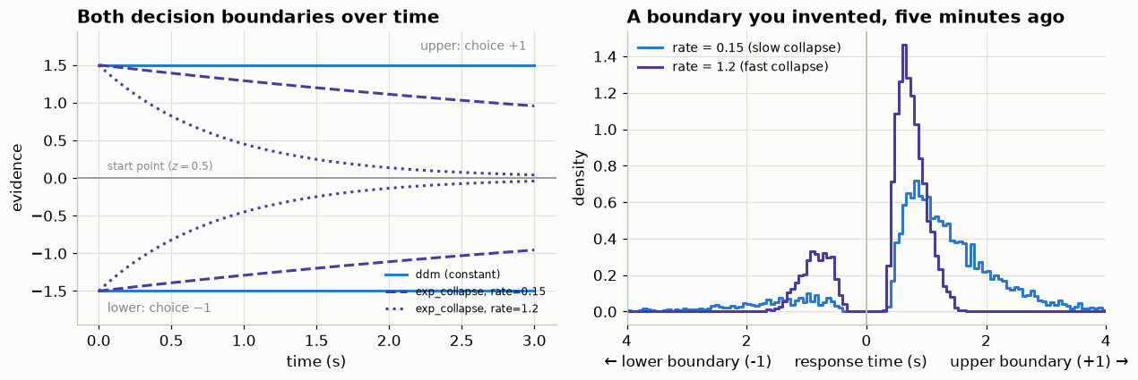

Read it exactly like the angle figure. On the left, the exponential decays toward zero rather than hitting it at a fixed time the way a linear collapse does — so there is always some evidence required, however long the trial runs. On the right, a faster collapse means less evidence is needed as time passes, so responses arrive sooner, and because the bound drops symmetrically the accuracy advantage shrinks with it: the fast-collapse curve is pulled toward zero on both sides and its two sides are closer in area.

Note the left panel is drawn by calling exp_collapse itself rather than by re-typing the formula. A figure that re-implements what it illustrates is one edit away from lying about it.

Check the boundary rather than trusting it

metadata["boundary"] is the boundary the simulator actually evaluated, on its internal time grid. Two things are worth reading off it, and the first settles the “is a applied twice?” question directly.

b = runs[RATES[0]]["metadata"]["boundary"]        # the slow-collapse run
print(f"b(0)  = {b[0]:.4f}      <- equals a = {A0} exactly, not {A0}^2 = {A0**2}")
print(f"b(t)  = {np.round(b[:4], 4)} ...")

# And it is the function we wrote, evaluated on that grid.
grid = np.arange(len(b)) * runs[RATES[0]]["metadata"]["delta_t"]
print("matches exp_collapse on the same grid:",
      np.allclose(b, exp_collapse(grid, a=A0, rate=RATES[0]), atol=1e-6))

b(0)  = 1.5000      <- equals a = 1.5 exactly, not 1.5^2 = 2.25
b(t)  = [1.5    1.4998 1.4996 1.4993] ...
matches exp_collapse on the same grid: True

⚠️ Not every engine honours a custom boundary

ddm, angle, weibull and the rest of the ddm_flexbound family evaluate your function on a time grid and walk against it. 13 of the 113 built-in models do not — ddm_legacy, addm, the whole LBA family, poisson_race and racing_diffusion_3. Their compiled simulators compute the bound internally and have no boundary_fun argument at all, so it lands in **kwargs and is discarded. You get no error, and usually no warning.

lba_angle_3 is the sharpest case: it declares boundary_name="constant", the config machinery dutifully routes a into the boundary call, and the engine ignores the lot. The config advertises support the engine lacks.

So build custom boundaries on a flexbound-family base model, and run the sweep above when you are unsure — it is three lines and it is the only way to tell. Reported upstream as ssm-simulators #310.

⚠️ Two ways a custom boundary goes wrong in silence

Leave the new parameter out of theta and it does not error — the simulator falls back to the Python default in your function signature, with no warning. {"v":…, "a":…, "z":…, "t":…} with no rate quietly simulates rate=0.5 because that is what def exp_collapse(t, a=1.0, rate=0.5) says. Misspell it in boundary_params and you get the same silence.

Leave it out of params — i.e. skip the three declaration overrides above — and dict-form theta still works perfectly, which is what makes this easy to miss. It breaks only when you pass theta as an array: ValueError: model_param_list and theta array do not imply the same number of parameters. validate_config does not catch it either way. Anything that reads the parameter box — priors, bounds, the ranges used to train a neural likelihood — will not see rate until you declare it. (ssm-simulators #308)

📝 The other route: registering a name

register_boundary("exp_collapse", exp_collapse, ["a", "rate"]) adds your function to a global registry, after which from_model(..., boundary_name=…) or ModelConfigBuilder.add_boundary(cfg, "exp_collapse") can find it by string. Useful when a boundary is shared across several configs.

We skipped it because it is a second concept that buys nothing here, and it has a trap: add_boundary(cfg, "name", ["a", "rate"]) silently ignores that third argument when the boundary is a string — the parameter list comes from the registry entry, so a list that disagrees with it is quietly discarded. The third argument is only read when you pass a callable.

The registry is also in-memory and per-process: restart the kernel and the name is gone. Passing the function object, as we did above, sidesteps all of this — and it survives multiprocessing just as well, because either way the function object ends up stored in the config that gets shipped to the worker.

One more reason to prefer the callable: add_boundary stores the registry’s own parameter list in your config rather than a copy, so an innocent cfg["boundary_params"].append(...) corrupts the registry for the rest of the process — and every later config built from that name inherits the damage. (ssm-simulators #311)

Route B — write the whole simulator

If your model is not a diffusion at all, hand over a function. It must accept the parameters you declare plus n_samples, and return a dict with rts, choices and metadata, where rts and choices are 2-D, shape (n_samples, 1).

def racing_exponentials(v0, v1, t, n_samples=1000, max_t=20.0, delta_t=0.001,
                        random_state=None, **kwargs):
    """Two exponential accumulators race; the first to finish picks the choice.

    Not a diffusion at all — the interface is genuinely open.
    """
    import numpy as np
    rng = np.random.default_rng(random_state)
    finish_0 = rng.exponential(1.0 / v0, n_samples)
    finish_1 = rng.exponential(1.0 / v1, n_samples)
    rts = (np.minimum(finish_0, finish_1) + t).reshape(-1, 1)
    choices = np.where(finish_1 < finish_0, 1, -1).reshape(-1, 1)
    return {"rts": rts, "choices": choices,
            "metadata": {"model": "racing_exponentials", "n_samples": n_samples}}


race = Simulator(simulator_function=racing_exponentials,
                 params=["v0", "v1", "t"], nchoices=2)
o = race.simulate(theta={"v0": 1.0, "v1": 2.0, "t": 0.25},
                  n_samples=3000, random_state=RANDOM_SEED)

rt_r, ch_r = np.asarray(o["rts"]).flatten(), np.asarray(o["choices"]).flatten()
print(f"P(choice = +1) = {(ch_r == 1).mean():.3f}   "
      f"(closed form v1/(v0+v1) = {2/3:.3f})")

fig, ax = plt.subplots(figsize=(7.0, 3.6))
lower, upper = S.signed_rt_hist(ax, rt_r, ch_r, rt_max=3.0,
                                color=S.PRIMARY, label="racing exponentials",
                                fill=False)
ax.set(title="A model that is not a diffusion", ylabel="density")
S.label_choice_axis(ax, rt_max=3.0,
                    lower="$-1$ (accumulator 0 won)",
                    upper="$+1$ (accumulator 1 won)")
ax.legend(loc="upper left", fontsize=9)
fig.tight_layout()

print(f"area on the +1 side = {upper:.3f}  (the closed form again)")

P(choice = +1) = 0.663   (closed form v1/(v0+v1) = 0.667)
area on the +1 side = 0.663  (the closed form again)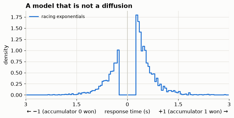

The analytic check matters: for two racing exponentials, \(P(\text{choice}=+1) = v_1/(v_0+v_1)\). We recovered it. If you find any close close-form quantity that your simulator should reproduce, check it! — it is the cheapest bug detector.

Exercise 2

Real response-time data almost always contains a few responses that the model did not generate: button mashing, attention lapses, a sneeze. Extend racing_exponentials with a contaminant process: with probability \(p_\text{lapse}\), a trial instead produces a uniform random RT in \([0, 3]\) s and a coin-flip choice.

Simulate with \(p_\text{lapse} = 0\) and \(p_\text{lapse} = 0.1\) and plot both. Where in the distribution does the contamination show up, and which part of it would you expect to distort a fit the most?

Solution, and why this parameter matters

def racing_with_lapse(v0, v1, t, p_lapse=0.0, n_samples=1000, max_t=20.0,
                      delta_t=0.001, random_state=None, **kwargs):
    import numpy as np
    rng = np.random.default_rng(random_state)
    f0 = rng.exponential(1.0 / v0, n_samples)
    f1 = rng.exponential(1.0 / v1, n_samples)
    rts = np.minimum(f0, f1) + t
    choices = np.where(f1 < f0, 1, -1)

    lapse = rng.random(n_samples) < p_lapse          # which trials are junk
    rts[lapse] = rng.uniform(0.0, 3.0, lapse.sum())
    choices[lapse] = rng.choice([-1, 1], lapse.sum())

    return {"rts": rts.reshape(-1, 1), "choices": choices.reshape(-1, 1),
            "metadata": {"model": "racing_with_lapse", "n_samples": n_samples}}

race_l = Simulator(simulator_function=racing_with_lapse,
                   params=["v0", "v1", "t", "p_lapse"], nchoices=2)

fig, ax = plt.subplots(figsize=(6.5, 3.6))
for p, colour in [(0.0, S.PRIMARY), (0.1, S.NAIVE)]:
    o = race_l.simulate(theta={"v0": 1.0, "v1": 2.0, "t": 0.25, "p_lapse": p},
                        n_samples=5000, random_state=0)
    ax.hist(np.asarray(o["rts"]).flatten(), bins=60, range=(0, 3), density=True,
            histtype="step", lw=2, color=colour, label=f"p_lapse = {p}")
ax.set(xlabel="RT (s)", ylabel="density"); ax.legend()

The contamination is nearly invisible in the bulk and obvious in the tails — it puts mass at very short RTs that the race process essentially never produces, and it fattens the slow tail. Those are exactly the regions a likelihood cares most about: a single impossibly-fast response can have a huge influence on the fit, because the model assigns it almost zero density.

This is not a toy concern. HSSM includes a lapse process by default — p_outlier=0.05 — for precisely this reason, and you will meet it tomorrow morning. Now you know what it is protecting you from.

5. The dataset for the next session

We hand two datasets forward. Same model, same number of trials — the only difference is the drift, and therefore the error rate.

import pandas as pd

def make_dataset(v, label, n=800, seed=RANDOM_SEED):
    o = sim.simulate(theta=[v, 1.2, 0.5, 0.3], n_samples=n, random_state=seed)
    return pd.DataFrame({"rt": o["rts"].flatten(),
                         "response": o["choices"].flatten().astype(int),
                         "design": label})

# v = 0.5 lands ~23% errors, inside the 15-35% band that Lüken et al. (2025)
# recommend for identifiability. v = 3.0 is the pathological case: ~0% errors.
balanced = make_dataset(0.5, "balanced")
extreme = make_dataset(3.0, "extreme")

for df in (balanced, extreme):
    err = (df["response"] == -1).mean()
    print(f"{df['design'][0]:9s} error rate {err:6.1%}   mean RT {df['rt'].mean():.3f}s")

outdir = pathlib.Path("data")
outdir.mkdir(exist_ok=True)
pd.concat([balanced, extreme]).to_csv(outdir / "ddm_two_designs.csv", index=False)
print(f"\nwrote {outdir / 'ddm_two_designs.csv'}")

balanced  error rate  22.9%   mean RT 1.579s
extreme   error rate   0.0%   mean RT 0.705s

wrote data/ddm_two_designs.csv

📝 Where this is going

Both datasets come from the same model with the same a, z, t. Only the drift differs. One of them supports clean parameter recovery and the other does not — and it is not the one most people would guess. That is the next session.

NOTE: data/ is gitignored: it is regenerated by running this notebook, never committed.

6. Other functionality (not less important, but we can only cover so much)

We stayed inside the two-choice diffusion family. The package goes considerably further, and two directions are worth knowing about:

Attentional drift-diffusion (addm) — drift depends on where the participant is looking on each moment of the trial, so fixation data enters the model directly. Use it when you have eye-tracking alongside choices and RTs.

Simulator(model="addm")   # takes per-trial fixation data via extra_fields

Reinforcement-learning SSMs (ssms.rl) — the drift rate on each trial is produced by a learning process, so choice, response time and learning are modelled jointly. This is how you fit a bandit task where you care about both what was learned and how the decision was made.

import ssms.rl                # learning rules that feed an SSM

Both plug into HSSM the same way the models here do. If your project involves eye-tracking or learning, start there rather than bolting it on later.

Training Data Generation - ssms has functionality to generate training data directly for multiple downstream amortization libraries (BayesFlow, LanFactory (holds our own network + trianing algorithms), sbi)

Quick reference

want to	call
build a simulator	sim = Simulator(model="ddm")
simulate	sim.simulate(theta=[...], n_samples=n)
list models	model_config.keys()
inspect one	model_config["angle"]
custom boundary	from_model("ddm", boundary=fn, boundary_params=["a", ...], params=[...])
check it took	out["metadata"]["boundary"]
bring your own simulator	Simulator(simulator_function=fn, params=[...], nchoices=2)

Next: we take the two datasets we just wrote and find out what happens when you try to recover the parameters that made them.