A tutorial on PyMC

Day 2, 12:00 — 60 minutes. Alexander Fengler.

PyMC lets you write a generative model in Python and get a posterior back. This session builds that from the bottom: what a distribution object is, what a model is made of, what pm.sample() actually hands you, and how to look at it. We finish by writing a regression twice — once by hand, once in one line with bambi — so you can see exactly what the shortcut is doing.

▶️ Running this on Google Colab

The cell below is a no-op on your own machine. On Colab it installs the stack and downloads the shared helper module, which lives one directory up in the repository and is therefore not importable there.

Expect the install to take a few minutes. If Colab asks you to restart the runtime, do it and then run the cell again — the second run is a no-op.

# --- Google Colab bootstrap; does nothing anywhere else ---------------------
import importlib.util, subprocess, sys, urllib.error, urllib.request

IN_COLAB = importlib.util.find_spec("google.colab") is not None

# `main` once this is merged; the branch is the fallback so the Colab path can
# be tested BEFORE the merge, when main does not yet have these files.
_REFS = ("main", "afengler.tutorials")
_RAW = "https://raw.githubusercontent.com/stefanradev93/sbi4cogsci/{ref}/tutorials/"


def _fetch(module):
    for ref in _REFS:
        try:
            urllib.request.urlretrieve(_RAW.format(ref=ref) + module, module)
            return ref
        except urllib.error.HTTPError:
            continue
    raise RuntimeError(f"could not fetch {module} from any of {_REFS}")


if IN_COLAB:
    # numba>=0.61 is REQUIRED, not cosmetic. pytensor resolves linker="auto" to
    # its numba backend, and numba renamed FunctionModel's first field
    # addr -> c_addr in 0.61. Colab preinstalls an older numba, and pytensor
    # declares numba only as an optional extra, so pip leaves it in place and
    # any MvNormal (SolveTriangular has no C implementation) dies with
    # KeyError: "FunctionModel does not have a field named 'c_addr'".
    subprocess.run([sys.executable, "-m", "pip", "install", "-q",
                    "numba>=0.61", "pymc>=6.2", "arviz>=1.2", "bambi>=0.19"],
                   check=True)
    # `dot` is a system binary, not a Python package.
    subprocess.run(["apt-get", "-qq", "install", "-y", "graphviz"],
                   check=True)
    for _mod in ["sbi4cogsci_style.py"]:
        print(f"  fetched {_mod} from {_fetch(_mod)}")
    print("Colab setup done.")

import sys, pathlib, warnings
sys.path.insert(0, str(pathlib.Path.cwd().parent))  # -> tutorials/

import numpy as np
import pandas as pd
import matplotlib.pyplot as plt
import pymc as pm
import arviz as az
import bambi as bmb
import sbi4cogsci_style as S

S.use()
warnings.filterwarnings("ignore")

RANDOM_SEED = sum(map(ord, "sbi4cogsci-pymc"))
rng = np.random.default_rng(RANDOM_SEED)

print("pymc", pm.__version__, "| arviz", az.__version__, "| bambi", bmb.__version__)

pymc 6.2.0 | arviz 1.2.0 | bambi 0.19.0

Where PyMC comes from, and what it actually does

PyMC is a probabilistic programming library. You write down a generative model — priors, then how data arise from them — and the library works out how to condition that model on observed data. You never write a sampler.

A very short history

PyMC has been developed since the mid-2000s, making it one of the older projects in this space. The version most people met, PyMC3, was built on Theano — an early symbolic-computation and automatic-differentiation library from the deep-learning world. When Theano’s upstream development wound down, the PyMC team took over maintenance and eventually forked it into what is now PyTensor, the engine under PyMC 5 and 6. That is an unusual situation worth knowing about: a statistics library ended up maintaining its own tensor and autodiff engine.

The idea it shares with deep learning frameworks

When you write

with pm.Model():
    mu = pm.Normal("mu", 0, 1)
    pm.Normal("y", mu=mu, sigma=1, observed=data)

nothing is computed yet. You are building a graph — a symbolic description of how quantities depend on one another. PyTensor can then

differentiate that graph automatically, and
compile it to fast code (C, numba, or JAX).

If you have used PyTorch or JAX, this is the same core machinery: define a computation graph, get gradients for free, compile it. What differs is what the gradients are for. In deep learning you differentiate a loss and descend it to a point estimate. Here you differentiate the log-posterior and hand those gradients to a sampler, which uses them to explore the posterior rather than to minimise anything. Same engine, different destination: the output is a distribution over parameters, not a fitted value.

The neighbourhood

	what it is
PyMC	the modelling library — this session
PyTensor	the graph / autodiff / compile engine underneath
ArviZ	diagnostics and plotting for whatever you fitted
bambi	common regressions as formulas; builds the PyMC model for you
nutpie	a fast NUTS implementation you can swap in
HSSM	sequential-sampling models on top of PyMC — Day 3, 09:30

Comparable tools elsewhere: Stan (its own language, very mature), NumPyro and Pyro (on JAX and PyTorch), Turing.jl (Julia). The concepts transfer directly; the syntax does not.

💡 The one sentence to keep

You describe the generative story; the library turns it into a differentiable (if feasible, non-differentiable is allowed) graph and samples the posterior for you.

⚠️ Read this before you copy code off the internet

ArviZ v1.0 (May 2026) was a breaking release. az.plot_posterior, az.plot_ppc, az.plot_density, az.plot_kde and az.waic no longer exist. az.plot_trace still exists but now draws traces only. The default credible interval changed from a 94% HDI to an 89% ETI, so even printed numbers differ from older material.

Most PyMC tutorials online — including large parts of PyMC’s own example gallery — predate this. If a snippet errors with AttributeError on an az.plot_* function, that is why. The pinned tutorials/uv.lock guarantees you are on the versions this notebook was written against.

1. What is a PyMC distribution?

Standalone

This is the piece most tutorials skip, and it is the source of a lot of early confusion. A PyMC distribution can be instantiated in primarily two different ways, and they behave differently.

# (a) Standalone — a distribution object, not attached to anything.
standalone = pm.Normal.dist(mu=0.0, sigma=1.0)
print("type:", type(standalone).__name__)
print("5 draws:", pm.draw(standalone, draws=5, random_seed=RANDOM_SEED).round(3))

type: TensorVariable
5 draws: [-0.241 -0.112 -0.713  0.371  0.275]

pm.Normal.dist(...) gives you a standalone distribution object. It doesn’t belong to any model. Use it whenever you want a distribution

as a value
inside another distribution
as a prior you are inspecting
just to simulate from a named distribution

Densities, not just draws

A distribution also knows its own log-density. This is the quantity every sampler in this course is actually working with.

grid = np.linspace(-4, 4, 9)
logp = pm.logp(standalone, grid).eval()

fig, ax = plt.subplots(figsize=(6.5, 3.2))
xs = np.linspace(-4, 4, 300)
ax.plot(xs, np.exp(pm.logp(pm.Normal.dist(0.0, 1.0), xs).eval()),
        color=S.PRIMARY, label="density")
ax.plot(grid, np.exp(logp), "o", color=S.PRIMARY, ms=6, ls="none")
ax.set(title="pm.logp evaluated on a grid", xlabel="$x$", ylabel="density")
ax.legend()
fig.tight_layout()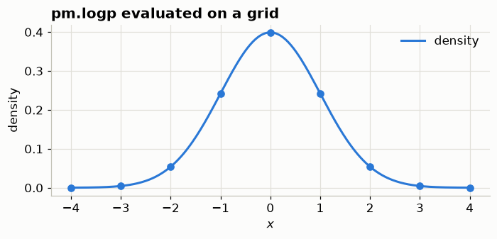

Now the second way:

Distributions inside a PyMC model

# (b) Named, inside a model context — a random VARIABLE in a graph.
with pm.Model() as demo:
    mu = pm.Normal("mu", mu=0.0, sigma=1.0)

print("type:", type(mu).__name__)
print("model variables:", [v.name for v in demo.basic_RVs])

# (b.1) Can now call it from the outside as well
print(pm.draw(demo.mu, draws = 10))

type: TensorVariable
model variables: ['mu']
[-0.08464932 -0.38373466 -0.38593725 -0.39279033 -0.42147142 -1.22132862
  0.01270711 -0.50015753  1.01399137 -0.49146933]

Inside a with pm.Model() block, the same call registers a node in a graph. The name is not decoration — it is the key you will use to get the posterior back out. Two variables cannot share a name.

Try it outside a model context and PyMC tells you exactly what is wrong:

try:
    oops = pm.Normal("mu", 0.0, 1.0)
except TypeError as e:
    print("TypeError:", e)

TypeError: No model on context stack, which is needed to instantiate distributions. Add variable inside a 'with model:' block, or use the '.dist' syntax for a standalone distribution.

Poll:
What is the difference between pm.Normal("x", 0, 1) and pm.Normal.dist(0, 1)?
- A. Nothing; .dist() is just shorthand.
- B. .dist() is faster because it skips validation.
- C. The named form registers a variable in the enclosing model; .dist() returns a free-standing distribution belonging to no model.
- D. .dist() can only be used for priors.

Answer

C. The named form needs a model context and will raise without one. The .dist() form is a value you can draw from, take the logp of, or nest inside another distribution — which is exactly how you build custom likelihoods and mixtures.

2. A first model, and what `pm.sample()` returns

The smallest interesting problem: we observe noisy measurements of an unknown mean and want the posterior over that mean. Written out,

\[ \mu \sim \text{Normal}(0,\ 10), \qquad \sigma \sim \text{HalfNormal}(5), \qquad y_i \mid \mu, \sigma \;\sim\; \text{Normal}(\mu,\ \sigma) \quad \text{for } i = 1,\dots,60 . \]

The first two lines are the prior, the third is the likelihood. The code below is a line-for-line transcription of exactly that.

TRUE_MU, TRUE_SIGMA, N = 2.5, 1.5, 60
y_obs = rng.normal(TRUE_MU, TRUE_SIGMA, N)

with pm.Model() as first_model:
    # Priors
    mu = pm.Normal("mu", mu=0.0, sigma=10.0)
    sigma = pm.HalfNormal("sigma", sigma=5.0)

    # Likelihood
    pm.Normal("y", mu=mu, sigma=sigma, observed=y_obs)

    # Posterior samples
    idata = pm.sample(draws=1000, tune=1000, chains=4, cores=1,
                      nuts_sampler="pymc", progressbar=False,
                      random_seed=RANDOM_SEED)

print(type(idata))

Initializing NUTS using jitter+adapt_diag...
Sequential sampling (4 chains in 1 job)
NUTS: [mu, sigma]
Sampling 4 chains for 1_000 tune and 1_000 draw iterations (4_000 + 4_000 draws total) took 0 seconds.

<class 'xarray.core.datatree.DataTree'>

Look at the model before you look at the answer

pm.model_to_graphviz draws the graph PyMC built. Shaded nodes are observed, open nodes are things being estimated, and the box is the plate — the 60 observations that share the same mu and sigma. Reading this before sampling catches an entire class of mistake: a prior you forgot to connect, a variable with the wrong shape, an observation that is not actually observed.

try:
    graph = pm.model_to_graphviz(first_model)
except Exception as exc:                      # graphviz needs the `dot` BINARY
    print(f"graphviz unavailable ({type(exc).__name__}); "
          "showing the mermaid description instead")
    print(pm.model_to_mermaid(first_model))
    graph = None
graph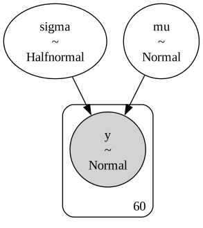

📝 If that cell printed text instead of a picture

model_to_graphviz needs the dot system binary, not just the Python graphviz package — brew install graphviz / apt install graphviz / conda install graphviz. PyMC 6 also ships pm.model_to_mermaid(), which is pure text and always available, which is what the fallback prints.

🔑 pm.sample() returns an xarray.DataTree

In PyMC 6 this is not an arviz.InferenceData any more. InferenceData still exists as a compatibility shim that warns and hands you a DataTree. The API docstring on the website still says “InferenceData” — the code disagrees, and the code wins.

A DataTree is a tree of labelled groups. Look at what is in it:

idata

list(idata.children)

['posterior', 'sample_stats', 'observed_data']


idata["posterior"].dataset

Data Structures that can cause confusion

idata.posterior is a DataTree node, not a Dataset. Most xarray operations you want live on the Dataset, so reach through via .dataset:

print("idata.posterior       ->", type(idata.posterior).__name__)
print("idata.posterior.dataset ->", type(idata.posterior.dataset).__name__)
print("idata.posterior['mu'] ->", type(idata.posterior["mu"]).__name__)
print()

post = idata.posterior.dataset
print("shape (chain, draw):", post["mu"].shape)
print("posterior mean mu = %.3f   (true %.1f)" % (post["mu"].values.mean(), TRUE_MU))
print("posterior mean sigma = %.3f (true %.1f)" % (post["sigma"].values.mean(), TRUE_SIGMA))

idata.posterior       -> DataTree
idata.posterior.dataset -> DatasetView
idata.posterior['mu'] -> DataArray

shape (chain, draw): (4, 1000)
posterior mean mu = 2.497   (true 2.5)
posterior mean sigma = 1.278 (true 1.5)

What you get once you are on the `Dataset`

It is worth being concrete about why that reach-through matters, because “use xarray” is advice people nod at and then ignore. The payoff is that the array carries its dimension names — chain, draw — so you stop writing axis=0 and start writing what you mean.

# 1. REDUCE BY NAME. No axis numbers, and it applies to every variable at once.
print(post.mean(dim=["chain", "draw"]))

<xarray.Dataset> Size: 16B
Dimensions:  ()
Data variables:
    mu       float64 8B 2.497
    sigma    float64 8B 1.278
Attributes:
    created_at:                 2026-07-28T17:17:37.978237+00:00
    creation_library:           ArviZ
    creation_library_version:   1.2.0
    creation_library_language:  Python
    inference_library:          pymc
    inference_library_version:  6.2.0
    sample_dims:                ['chain', 'draw']
    sampling_time:              0.3696708679199219
    tuning_steps:               1000

# 2. SELECT BY LABEL. `sel` uses coordinate values, `isel` uses positions.
#    "chain 2, last five draws" is one expression rather than a slice puzzle.
print("chain 2, last 5 draws of mu:",
      post["mu"].sel(chain=2).isel(draw=slice(-5, None)).values.round(3))

chain 2, last 5 draws of mu: [2.866 2.404 2.514 2.515 2.795]

# 3. PER-CHAIN MEANS
print("mean of mu within each chain:")
print(post["mu"].mean(dim="draw").to_series().round(3).to_string())

mean of mu within each chain:
chain
0    2.489
1    2.497
2    2.500
3    2.501

# 4. DERIVED QUANTITIES ARE FREE, and stay labelled. Any function of the
#    parameters has a posterior too, and you get it by transforming the draws --
#    no re-fitting, no delta method, no reshaping.
derived = post.assign(
    cv=post["sigma"] / post["mu"],            # coefficient of variation
    z_score=(3.0 - post["mu"]) / post["sigma"],  # how extreme is y = 3?
)
print(az.summary(derived, var_names=["cv", "z_score"], kind="stats").to_string())

         mean    sd eti89_lb eti89_ub
cv       0.51  0.06     0.43     0.62
z_score   0.4  0.14     0.19     0.62

# 5. QUANTILES ALONG NAMED DIMS. `az.summary` is the convenient path, but the
#    raw xarray call is there when you want something it does not offer.
print(post.quantile([0.055, 0.5, 0.945], dim=["chain", "draw"])
          .to_dataframe().round(3).to_string())

             mu  sigma
quantile              
0.055     2.233  1.098
0.500     2.498  1.270
0.945     2.763  1.481

Point 3 is the one to remember. The posterior over \(\sigma/\mu\) was never something we asked the sampler for — we pushed the draws through a function and read off the answer. Any quantity you can compute from the parameters has a posterior, and this is how you get it. That is a genuine advantage of sampling over optimisation, where propagating uncertainty through a nonlinear transform is real work.

The sample_stats group is where the sampler records what it did. This is where divergences live — we will make use of it during out Day 3 tutorials.

print(sorted(idata["sample_stats"].dataset.data_vars))

['acceptance_rate', 'divergences', 'diverging', 'energy', 'energy_error', 'index_in_trajectory', 'largest_eigval', 'lp', 'max_energy_error', 'n_steps', 'perf_counter_diff', 'perf_counter_start', 'process_time_diff', 'reached_max_treedepth', 'smallest_eigval', 'step_size', 'step_size_bar', 'tree_depth']

`coords` and `dims` — naming your own dimensions

Everything above worked because chain and draw are named dimensions. You can name your parameters’ dimensions too, and once a model has more than one of anything — one drift per condition, one intercept per participant — you will want to.

The alternative is shape=, which works but leaves the result anonymous. Compare. Three group means, three observations each:

y_grp = rng.normal([1.0, 2.0, 3.0], 1.0, size=(40, 3))

# (a) shape= — correct, but the posterior does not know what the axis MEANS
with pm.Model() as m_shape:
    mu_s = pm.Normal("mu", 0.0, 5.0, shape=3)
    pm.Normal("y", mu=mu_s, sigma=1.0, observed=y_grp)
    idata_shape = pm.sample(300,
                            tune=300, 
                            chains=2,
                            cores=1,
                            nuts_sampler="pymc",
                            progressbar=False,
                            random_seed=RANDOM_SEED
                            )

print("\n \n dimension names:", list(idata_shape.posterior.dataset["mu"].dims))
print(az.summary(idata_shape, kind="stats").to_string())

Initializing NUTS using jitter+adapt_diag...
Sequential sampling (2 chains in 1 job)
NUTS: [mu]
Sampling 2 chains for 300 tune and 300 draw iterations (600 + 600 draws total) took 0 seconds.
We recommend running at least 4 chains for robust computation of convergence diagnostics


 
 dimension names: ['chain', 'draw', 'mu_dim_0']
       mean    sd eti89_lb eti89_ub
mu[0]  0.93  0.16     0.69      1.2
mu[1]   1.9  0.16      1.7      2.2
mu[2]     3  0.17      2.8      3.3

# (b) coords + dims — the model carries the labels, and so does everything after
COORDS = {"condition": ["low", "med", "high"]}

with pm.Model(coords=COORDS) as m_dims:
    mu_d = pm.Normal("mu", 0.0, 5.0, dims="condition")
    pm.Normal("y", mu=mu_d, sigma=1.0, observed=y_grp)
    idata_dims = pm.sample(300,
                           tune=300,
                           chains=2,
                           cores=1,
                           nuts_sampler="pymc",
                           progressbar=False,
                           random_seed=RANDOM_SEED
                           )

print("\n \ndimension names:", list(idata_dims.posterior.dataset["mu"].dims))
print(az.summary(idata_dims, kind="stats").to_string())

Initializing NUTS using jitter+adapt_diag...
Sequential sampling (2 chains in 1 job)
NUTS: [mu]
Sampling 2 chains for 300 tune and 300 draw iterations (600 + 600 draws total) took 0 seconds.
We recommend running at least 4 chains for robust computation of convergence diagnostics


 
dimension names: ['chain', 'draw', 'condition']
          mean    sd eti89_lb eti89_ub
mu[low]   0.93  0.16     0.69      1.2
mu[med]    1.9  0.16      1.7      2.2
mu[high]     3  0.17      2.8      3.3

mu[0], mu[1], mu[2] became mu[low], mu[med], mu[high]. That is not cosmetic — the labels are now data you can compute with:

post_d = idata_dims.posterior.dataset
print("the 'high' condition only:",
      round(float(post_d["mu"].sel(condition="high").mean()), 3))

# A contrast, by name rather than by remembering which integer is which.
contrast = post_d["mu"].sel(condition="high") - post_d["mu"].sel(condition="low")
print(f"high - low = {float(contrast.mean()):.3f} "
      f"[{float(contrast.quantile(0.055)):.3f}, {float(contrast.quantile(0.945)):.3f}]")

the 'high' condition only: 3.033
high - low = 2.100 [1.717, 2.497]

💡 Why this matters more than it looks

Three reasons to reach for dims from the start:

You stop counting indices. sel(condition="high") cannot silently become the wrong group the way [2] can when you reorder a list.
Plots and tables label themselves. az.summary, az.plot_forest and the rest read the coordinate values, so figures arrive with real names on them instead of mu[0].
It is what the libraries above PyMC do anyway. Every posterior you see for the rest of this course is labelled this way — at 14:30 you will write pm.Model(coords=...) with dims="coherence" for a drift rate per coherence level, and tomorrow HSSM will hand you back a_C(cond)[hard] without you asking. Recognising where those labels come from is the point of this section.

The cost is one dictionary. pm.Model(coords={"condition": [...]}) declares the labels once; dims="condition" on a variable adopts them and sets its shape for you — note we never wrote shape=3 in the second model.

3. Looking at a posterior

print(az.summary(idata, kind="stats").to_string())

      mean    sd eti89_lb eti89_ub
mu     2.5  0.17      2.2      2.8
sigma  1.3  0.12      1.1      1.5

Note the interval columns: 89% ETI, not the 94% HDI you may remember. You can ask for something else explicitly:

print(az.summary(idata, kind="stats", ci_prob=0.94, ci_kind="hdi").to_string())

      mean    sd hdi94_lb hdi94_ub
mu     2.5  0.17      2.2      2.8
sigma  1.3  0.12      1.1      1.5

The standard first look is plot_trace_dist — marginals on the left, traces on the right.

trace = az.plot_trace_dist(idata, combined=True)
plt.gcf().set_size_inches(9, 4.4)

# ArviZ returns a PlotCollection rather than an array of Axes. `get_target`
# takes the variable and the panel's coordinates and hands back the Axes, which
# is how we draw anything ArviZ does not — here, the values we generated from.
# The marginal panel wants a VERTICAL truth line (the x axis is the parameter);
# the trace panel wants a HORIZONTAL one (the y axis is the parameter).
for var, truth in [("mu", TRUE_MU), ("sigma", TRUE_SIGMA)]:
    S.truth_line(trace.get_target(var, {"column": "dist"}), truth, axis="x")
    S.truth_line(trace.get_target(var, {"column": "trace"}), truth, axis="y")

plt.tight_layout()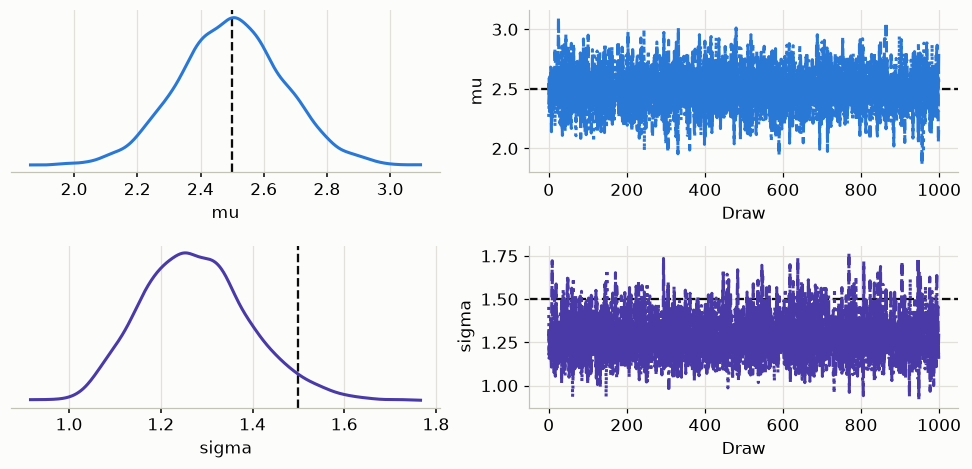

On the left it tells you whether the posterior actually covers the value that generated the data. On the right it tells you whether the chains are wandering around that value rather than drifting toward it — a trace that approaches the truth from one side and keeps going is a chain that has not converged.

And the joint, az.plot_pair gives the marginals on the diagonal and the joint off it. marginal_kind="kde" smooths the marginals into densities rather than histograms.

pair = az.plot_pair(idata, var_names=["mu", "sigma"],
                    marginal=True, marginal_kind="kde")

# ArviZ returns a PlotMatrix, not a bare matplotlib figure. `get_target` hands
# back the Axes for a given panel, which is how we add anything ArviZ does not
# draw itself — here, the true values used to generate the data.
S.truth_point(pair.get_target("mu", {}, "sigma", {}), TRUE_MU, TRUE_SIGMA)
for var, truth in [("mu", TRUE_MU), ("sigma", TRUE_SIGMA)]:
    pair.get_target(var, {}).axvline(truth, color=S.TRUTH, ls="--", lw=1.5)

plt.gcf().suptitle("Joint posterior, truth marked", y=1.02)
plt.tight_layout()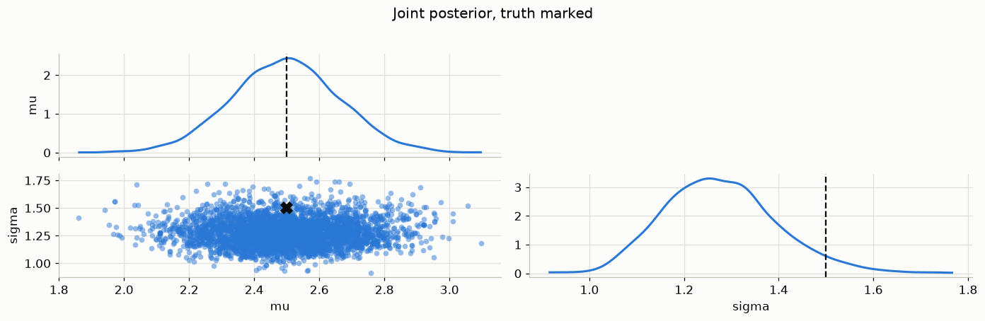

📝 Marking ground truth is a habit worth forming

ArviZ has no “true value” argument, because in real analyses there is no true value to pass — you only have this when you generated the data yourself. That is exactly why it is worth doing whenever you can: a plot with the truth on it answers “did this work?” in one glance, and simulating data with known parameters is the cheapest way to check a model before trusting it on real data. We use the same trick throughout Day 2 and Day 3.

mu and sigma are close to independent here — a round blob, and the truth sits inside it. Remember what this looks like; by 15:00 today you will be looking at one that is not.

What conditioning on data actually did

Two pictures make the whole point of Bayesian inference concrete. Both compare before seeing the data with after.

Prior to posterior is contraction in parameter space: the prior says what we were willing to believe, the posterior says what survives contact with 60 observations.

with first_model:
    prior = pm.sample_prior_predictive(draws=2000, random_seed=RANDOM_SEED)

# Two rows: the top shows the contraction, the bottom zooms in so the posterior
# is more than a spike. Both are needed — the first is the message, the second
# is the shape.
fig, axes = plt.subplots(2, 2, figsize=(11, 6.4))
for col, (var, truth) in enumerate([("mu", TRUE_MU), ("sigma", TRUE_SIGMA)]):
    pri = prior["prior"].dataset[var].values.ravel()
    pos = post[var].values.ravel()

    # top: full prior range
    ax = axes[0, col]
    lo, hi = np.percentile(pri, [0.5, 99.5])
    bins = np.linspace(lo, hi, 70)
    ax.hist(pri, bins=bins, density=True, color=S.MUTED, alpha=0.6, label="prior")
    ax.hist(pos, bins=bins, density=True, color=S.PRIMARY, label="posterior")
    S.truth_line(ax, truth, axis="x")
    ax.set(title=f"${var}$ — on the prior's scale", ylabel="density")
    ax.legend(fontsize=9)

    # bottom: zoomed to the posterior
    ax = axes[1, col]
    zlo, zhi = np.percentile(pos, [0.1, 99.9])
    pad = 0.35 * (zhi - zlo)
    zbins = np.linspace(zlo - pad, zhi + pad, 60)
    ax.hist(pos, bins=zbins, density=True, color=S.PRIMARY, label="posterior")
    S.truth_line(ax, truth, axis="x")
    ax.set(title=f"${var}$ — zoomed to the posterior", xlabel=f"${var}$",
           ylabel="density")
    ax.legend(fontsize=9)

    shrink = pri.std() / pos.std()
    axes[0, col].annotate(f"{shrink:.0f}x narrower", xy=(0.97, 0.75),
                          xycoords="axes fraction", ha="right",
                          color=S.PRIMARY, fontweight="bold")
fig.tight_layout()

for var in ["mu", "sigma"]:
    pri = prior["prior"].dataset[var].values.ravel()
    pos = post[var].values.ravel()
    print(f"sd({var}): prior {pri.std():7.3f} -> posterior {pos.std():6.3f}"
          f"   ({pri.std()/pos.std():.0f}x narrower)")

Sampling: [mu, sigma, y]

sd(mu): prior  10.032 -> posterior  0.166   (60x narrower)
sd(sigma): prior   2.942 -> posterior  0.120   (25x narrower)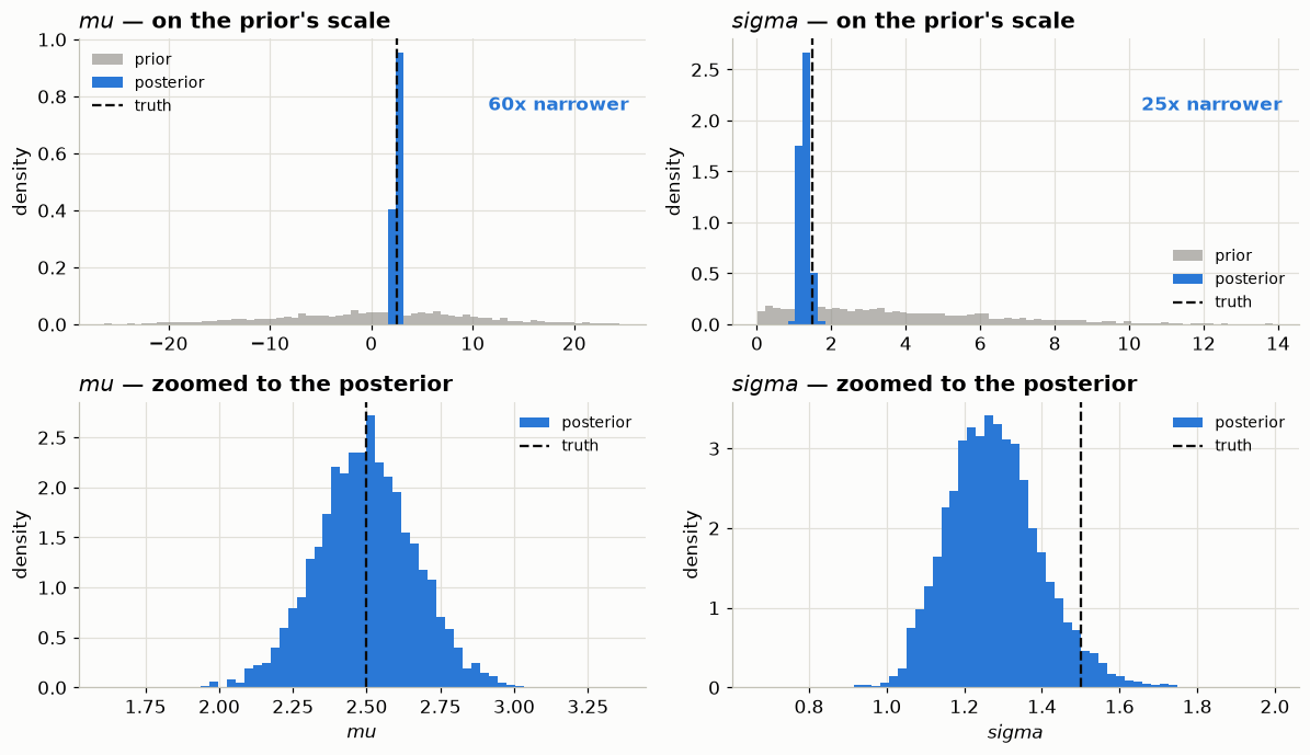

The posterior is dramatically narrower than the prior. That narrowing is the information the data carried — and it is why “what is your prior?” and “how wide is it?” are really the same question.

Look at the bottom-right panel before moving on: the true \(\sigma = 1.5\) sits in the right tail of its posterior, not in the middle. With 60 observations that is ordinary sampling variability, not a bug — a 89% interval misses the truth roughly 11% of the time, by construction. Being calibrated does not mean being right every time, and a posterior that always covered the truth dead-centre would be a suspiciously overconfident one.

Prior predictive to posterior predictive is the same story in data space: what datasets did the model consider plausible before and after?

with first_model:
    ppc = pm.sample_posterior_predictive(idata, random_seed=RANDOM_SEED,
                                         progressbar=False)

fig, ax = plt.subplots(figsize=(7, 4))
bins = np.linspace(-25, 30, 90)
ax.hist(prior["prior_predictive"].dataset["y"].values.ravel(), bins=bins,
        density=True, color=S.MUTED, alpha=0.55, label="prior predictive")
ax.hist(ppc["posterior_predictive"].dataset["y"].values.ravel(), bins=bins,
        density=True, color=S.PRIMARY, alpha=0.8, label="posterior predictive")
ax.plot(y_obs, np.full_like(y_obs, -0.004), "|", color=S.TRUTH, ms=12,
        label="observed data")
ax.set(title="Which datasets did the model think were plausible?",
       xlabel="$y$", ylabel="density")
ax.legend()
fig.tight_layout()

Sampling: [y]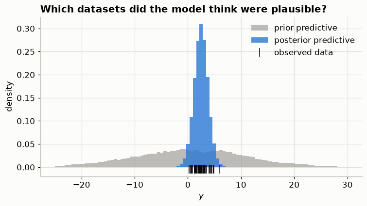

Before seeing anything, the model was prepared for data anywhere across a very wide range — that is the Normal(0, 10) prior on mu talking. Afterwards it predicts data that look like what we actually observed.

💡 These are two different checks, and both are worth running

The prior predictive is checked before fitting and asks “is my model capable of producing data like mine at all?” The posterior predictive is checked after and asks “having fitted, can it reproduce what I saw?” A model can pass the second and still have had an absurd prior — which is why the first is not optional.

Exercise 1

Re-fit first_model with a deliberately bad prior on mu — say pm.Normal("mu", 20, 0.5) — and compare the posterior mean to the truth. How much does 60 data points overcome a confidently wrong prior?

Solution

with pm.Model():
    mu = pm.Normal("mu", 20.0, 0.5)          # confidently wrong
    sigma = pm.HalfNormal("sigma", 5.0)
    pm.Normal("y", mu=mu, sigma=sigma, observed=y_obs)
    bad = pm.sample(draws=1000, tune=1000, chains=4, cores=1,
                    nuts_sampler="pymc", progressbar=False,
                    random_seed=RANDOM_SEED)
print(az.summary(bad, kind="stats").to_string())

The posterior lands between the prior and the data, much nearer the prior than you might like — a sigma=0.5 prior is worth a lot of observations. The lesson is not “priors are dangerous” but “a prior is a claim, and you should be able to defend its width as readily as its centre.”

Exercise 2

The Normal was an example, not the point. The machinery is identical for any distribution PyMC knows. Fit a Gamma:

\[ \alpha \sim \text{HalfNormal}(5), \qquad \beta \sim \text{HalfNormal}(5), \qquad y_i \mid \alpha, \beta \;\sim\; \text{Gamma}(\alpha,\ \beta). \]

Generate data from pm.draw(pm.Gamma.dist(alpha=3.0, beta=2.0), 200), build the model, sample it, and check that the posterior covers \(\alpha = 3\) and \(\beta = 2\). Then plot the joint with az.plot_pair and mark the truth as we did above.

Solution

TRUE_ALPHA, TRUE_BETA = 3.0, 2.0
y_gamma = pm.draw(pm.Gamma.dist(alpha=TRUE_ALPHA, beta=TRUE_BETA), 200,
                  random_seed=RANDOM_SEED)

with pm.Model() as gamma_model:
    alpha = pm.HalfNormal("alpha", 5.0)
    beta = pm.HalfNormal("beta", 5.0)
    pm.Gamma("y", alpha=alpha, beta=beta, observed=y_gamma)
    idata_gamma = pm.sample(draws=1000, tune=1000, chains=4, cores=1,
                            nuts_sampler="pymc", progressbar=False,
                            random_seed=RANDOM_SEED)

print(az.summary(idata_gamma, kind="stats").to_string())

pair_g = az.plot_pair(idata_gamma, var_names=["alpha", "beta"],
                      marginal=True, marginal_kind="kde")
S.truth_point(pair_g.get_target("alpha", {}, "beta", {}), TRUE_ALPHA, TRUE_BETA)

Two things to notice. First, nothing about the workflow changed — swap the distribution, keep everything else. Second, the joint posterior of alpha and beta is not a round blob: they are strongly positively correlated, because the Gamma’s mean is \(\alpha/\beta\) and the data pin the mean down much better than they pin down either parameter alone. You have just found a parameter trade-off, three hours before the session about them.

4. A regression, by hand

Same machinery, one step up:

\[ \beta_0 \sim \text{Normal}(0,\ 5), \qquad \beta_1 \sim \text{Normal}(0,\ 5), \qquad \sigma \sim \text{HalfNormal}(5), \] \[ y_i \mid \beta_0, \beta_1, \sigma \;\sim\; \text{Normal}(\beta_0 + \beta_1 x_i,\ \sigma). \]

Only the mean changed: it is now a function of a covariate instead of a single number. Everything else — priors, likelihood, sampling, diagnostics — is what you already saw.

# Generate Data
N_DATA = 120
rng = np.random.default_rng(RANDOM_SEED)

x = rng.normal(0.0, 1.0, N_DATA)
TRUE_INTERCEPT, TRUE_SLOPE, TRUE_NOISE = 1.0, 2.0, 0.8
y = TRUE_INTERCEPT + TRUE_SLOPE * x + rng.normal(0.0, TRUE_NOISE, N_DATA)
data = pd.DataFrame({"x": x, "y": y})

with pm.Model() as regression:
    # Priors
    intercept = pm.Normal("Intercept", 0.0, 5.0)
    slope = pm.Normal("x", 0.0, 5.0)
    sigma = pm.HalfNormal("sigma", 5.0)

    # Likelihood
    pm.Normal("y", mu=intercept + slope * data["x"].to_numpy(), sigma=sigma,
              observed=data["y"].to_numpy())

    # Sample
    idata_pymc = pm.sample(draws=1000, tune=1000, chains=4, cores=1,
                           nuts_sampler="pymc", progressbar=True,
                           random_seed=RANDOM_SEED)

print(az.summary(idata_pymc, kind="stats").to_string())
print(f"\ntruth: Intercept={TRUE_INTERCEPT}, x={TRUE_SLOPE}, sigma={TRUE_NOISE}")

Initializing NUTS using jitter+adapt_diag...
Sequential sampling (4 chains in 1 job)
NUTS: [Intercept, x, sigma]

Sampling 4 chains for 1_000 tune and 1_000 draw iterations (4_000 + 4_000 draws total) took 1 seconds.

           mean     sd eti89_lb eti89_ub
Intercept  0.96  0.072     0.85      1.1
x           1.9  0.079      1.8      2.1
sigma      0.78  0.051      0.7     0.86

truth: Intercept=1.0, x=2.0, sigma=0.8

Four lines of model, and every line is a modelling decision you made on purpose. That is the virtue of writing it out.

# Extract the posterior samples as an xarray dataset
post_p = idata_pymc.posterior.dataset

# Create a dense grid of x values spanning the observed data
xs = np.linspace(x.min(), x.max(), 100)

# Randomly sample 60 draws from the posterior (without replacement)
# This is for visualizing plausible regression lines
draws = rng.choice(post_p["Intercept"].values.size, 60, replace=False)

# Extract the sampled intercept and slope values (flatten to 1D)
ic = post_p["Intercept"].values.ravel()[draws]
sl = post_p["x"].values.ravel()[draws]

# Initialize the plot
fig, ax = plt.subplots(figsize=(6.5, 4))

# Plot 60 regression lines corresponding to random posterior draws
# These demonstrate plausible regression solutions the model considers likely
for i, s in zip(ic, sl):
    ax.plot(xs, i + s * xs, color=S.PRIMARY, alpha=0.12, lw=1)

# Plot the observed data points
ax.plot(
    x, y, 
    "o",                     # Marker style
    color=S.MUTED,           # Color for data
    ms=4,                    # Marker size
    ls="none",               # No connecting lines
    label="data", 
    zorder=3
)

# Plot the true underlying regression line used to generate the data
ax.plot(
    xs, TRUE_INTERCEPT + TRUE_SLOPE * xs,
    "--",                    # Dashed line for the true regression
    color=S.TRUTH,
    lw=1.8,
    label="truth", 
    zorder=4
)

# Add a dummy line for the legend to clarify which lines are posterior samples
ax.plot([], [], color=S.PRIMARY, alpha=0.5, label="posterior draws")

# Add axis labels and a title
ax.set(
    title="Posterior over regression lines", 
    xlabel="$x$", 
    ylabel="$y$"
)
ax.legend()                   # Add legend
fig.tight_layout()            # Format the layout tightly for clarity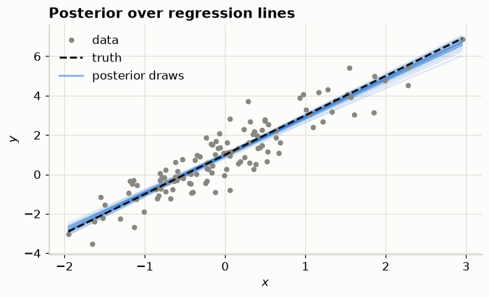

Two bands that are not the same thing

The plot above was assembled by hand: pull draws, multiply them out, draw lines. PyMC will do predictions for you with sample_posterior_predictive — but what it gives back answers a different question, and the two get conflated constantly. Name them properly:

	what it is	what it contains
mean band	uncertainty about \(\mu(x) = \beta_0 + \beta_1 x\) — where the line is	uncertainty in the coefficients only
response band	uncertainty about a new observation \(y^{\text{new}}\) at \(x\)	the coefficients plus the scatter \(\sigma\) around the line

In one equation, the widths differ by exactly one term:

\[ \operatorname{Var}\!\left(y^{\text{new}} \mid x\right) \;=\; \underbrace{\operatorname{Var}(\mu(x))}_{\text{mean band}} \;+\; \underbrace{\sigma^2}_{\text{observation noise}} . \]

The regression lines you just drew are the mean band. What sample_posterior_predictive returns is the response band. Let us compute both and put them on the same axes, because the comparison is the lesson.

# MEAN band: push the coefficient draws through the line. No noise anywhere.
ic_all = post_p["Intercept"].values.ravel()
sl_all = post_p["x"].values.ravel()
sd_all = post_p["sigma"].values.ravel()
mu_draws = ic_all[:, None] + sl_all[:, None] * xs[None, :]      # (draws, grid)
mu_lo, mu_mid, mu_hi = np.percentile(mu_draws, [5.5, 50, 94.5], axis=0)

# RESPONSE band, built BY HAND on the same grid so the two are comparable:
# take each posterior line and scatter a point around it with that draw's sigma.
# This is literally the definition, and doing it explicitly is the point.
rng_pp = np.random.default_rng(RANDOM_SEED)
y_new_draws = mu_draws + rng_pp.normal(0.0, 1.0, mu_draws.shape) * sd_all[:, None]
y_lo, y_hi = np.percentile(y_new_draws, [5.5, 94.5], axis=0)

# ...and the same thing from PyMC, at the x values the model was BUILT with.
with regression:
    ppc_reg = pm.sample_posterior_predictive(idata_pymc, random_seed=RANDOM_SEED,
                                             progressbar=False)

y_pred = ppc_reg["posterior_predictive"].dataset["y"].values   # (chain, draw, obs)
y_pred = y_pred.reshape(-1, y_pred.shape[-1])
lo, mid, hi = np.percentile(y_pred, [5.5, 50, 94.5], axis=0)
order = np.argsort(x)

fig, axes = plt.subplots(1, 3, figsize=(14.5, 4.1))

# (1) The mean band alone, zoomed so the hourglass is actually visible.
ax = axes[0]
ax.fill_between(xs, mu_lo, mu_hi, color=S.PRIMARY, alpha=0.40,
                label="89% band for the MEAN")
ax.plot(xs, mu_mid, color=S.PRIMARY, lw=1.5)
ax.plot(x, y, "o", color=S.MUTED, ms=3, ls="none", alpha=0.45, zorder=1)
pad = 3.5 * (mu_hi - mu_lo).max()
ax.set(title="Where is the line?", xlabel="$x$", ylabel="$y$",
       ylim=(mu_mid.min() - pad, mu_mid.max() + pad))
ax.legend(fontsize=9, loc="upper left")

# (2) Both bands, to scale.
ax = axes[1]
ax.fill_between(x[order], lo[order], hi[order], color=S.ALT, alpha=0.25,
                label="89% for a NEW OBSERVATION")
ax.fill_between(xs, mu_lo, mu_hi, color=S.PRIMARY, alpha=0.60,
                label="89% for the MEAN")
ax.plot(x, y, "o", color=S.MUTED, ms=4, ls="none", label="data", zorder=3)
ax.set(title="...versus the next data point?", xlabel="$x$")
ax.legend(fontsize=9, loc="upper left")

# (3) The diagnostic: each band's width RELATIVE TO ITS OWN NARROWEST POINT.
#     Both start at 1.0, so the comparison is about shape, not scale.
ax = axes[2]
w_mu = mu_hi - mu_lo
w_y = y_hi - y_lo
ax.plot(xs, w_mu / w_mu.min(), color=S.PRIMARY, lw=2.5, label="MEAN band")
ax.plot(xs, w_y / w_y.min(), color=S.ALT, lw=2.5, label="RESPONSE band")
S.truth_line(ax, 1.0, label="no flare at all")
ax.set(title="How much does each band flare?", xlabel="$x$",
       ylabel="width / narrowest width")
ax.legend(fontsize=9)
fig.tight_layout()

Sampling: [y]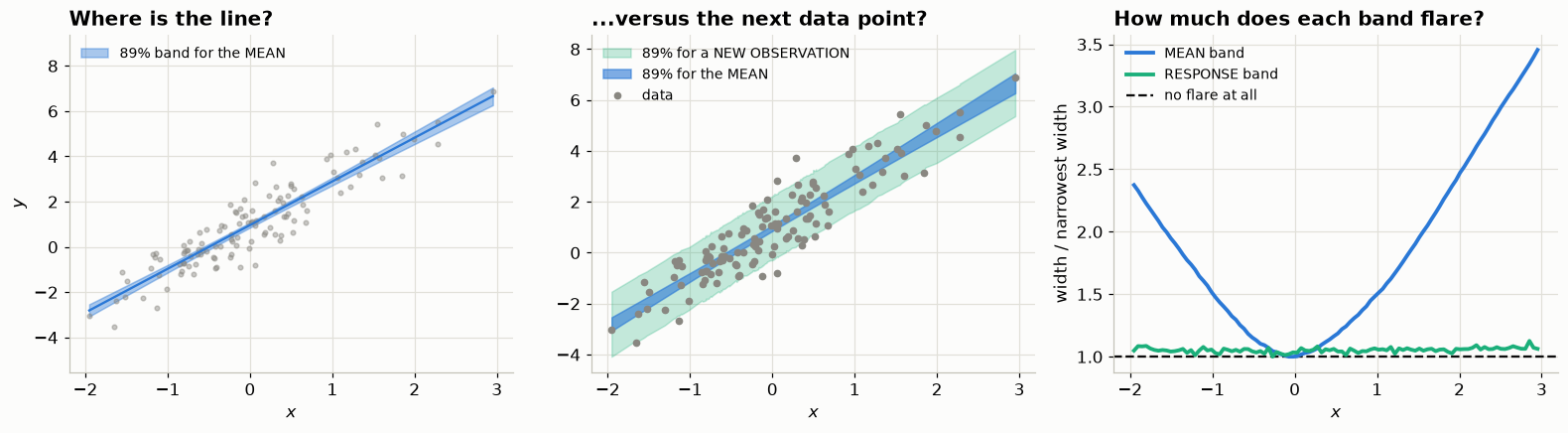

Why the wide band looks like it has constant width

It is worth checking that suspicion with numbers rather than eyes. The mean band is narrowest at the centre of the \(x\) range and flares at the extremes — the classic hourglass, because tilting the line about its centre moves the ends far more than the middle. The response band inherits that same hourglass, but adds \(\sigma^2\) to the variance, and here \(\sigma \approx 0.8\) dwarfs the coefficient uncertainty. So it is not flat — it is an hourglass swamped by a constant.

centre = np.argmin(np.abs(xs))                 # grid point nearest x = 0
edge = -1                                      # the largest x

mean_w = mu_hi - mu_lo
resp_w = y_hi - y_lo                           # both on the same grid now

print(f"{'':22s} {'at x ~ 0':>10s} {'at x = max':>12s} {'ratio':>8s}")
print(f"{'mean band width':22s} {mean_w[centre]:10.3f} {mean_w[edge]:12.3f}"
      f" {mean_w[edge] / mean_w[centre]:8.2f}")
print(f"{'response band width':22s} {resp_w[centre]:10.3f} {resp_w[edge]:12.3f}"
      f" {resp_w[edge] / resp_w[centre]:8.2f}")

# Sanity check: our hand-built response band and PyMC's should agree, since
# they are the same definition. Compare at the observed x, where PyMC has one.
pymc_w = np.interp(x[order], xs, resp_w)
print(f"\nhand-built vs pm.sample_posterior_predictive band width: "
      f"max gap {np.abs(pymc_w - (hi - lo)[order]).max():.3f}")

# The variance decomposition, at both ends. Standard deviations add IN
# QUADRATURE, which is the whole reason the flare gets flattened.
sigma_hat = post_p["sigma"].values.mean()
print(f"\nsigma = {sigma_hat:.3f}")
print(f"\n{'':10s} {'sd of mean':>11s} {'total sd':>10s}   decomposition")
for label, j in [("at x ~ 0", centre), ("at x = max", -1)]:
    sd_mu = mu_draws[:, j].std()
    total = np.sqrt(sd_mu**2 + sigma_hat**2)
    print(f"{label:10s} {sd_mu:11.3f} {total:10.3f}   "
          f"sqrt({sd_mu:.3f}^2 + {sigma_hat:.3f}^2)")

sd_c, sd_e = mu_draws[:, centre].std(), mu_draws[:, -1].std()
print(f"\nthe mean's sd grows {sd_e / sd_c:.2f}x from centre to edge,")
print(f"but the total sd grows only "
      f"{np.sqrt(sd_e**2 + sigma_hat**2) / np.sqrt(sd_c**2 + sigma_hat**2):.2f}x")
print(f"-> at the centre, noise is "
      f"{sigma_hat**2 / (sd_c**2 + sigma_hat**2):.1%} of the total variance")

                         at x ~ 0   at x = max    ratio
mean band width             0.225        0.778     3.45
response band width         2.470        2.538     1.03

hand-built vs pm.sample_posterior_predictive band width: max gap 0.124

sigma = 0.775

            sd of mean   total sd   decomposition
at x ~ 0         0.072      0.779   sqrt(0.072^2 + 0.775^2)
at x = max       0.243      0.812   sqrt(0.243^2 + 0.775^2)

the mean's sd grows 3.39x from centre to edge,
but the total sd grows only 1.04x
-> at the centre, noise is 99.2% of the total variance

There it is — the third panel is the whole answer. The mean band’s width more than triples from centre to edge; the response band’s sits flat on 1.0.

The mechanism is worth stating exactly, because it is easy to get half-right. The response band does inherit the flare, but standard deviations combine in quadrature, not additively:

\[ \operatorname{sd}\!\left(y^{\text{new}} \mid x\right) = \sqrt{\operatorname{sd}(\mu(x))^2 + \sigma^2}. \]

When \(\sigma\) is much the larger term, adding a small quantity under a square root barely moves the result — which is why the ratios printed above differ so sharply while describing the same underlying flare. The flare is not absent, it is ** suppressed**. So the suspicion that the wide band has constant width is a good one, and the resolution is that it very nearly does, for a reason.

(The small wobble on the green curve is Monte Carlo noise in the percentiles, not structure. More draws would flatten it further.)

This is a fact about this dataset, not about regression. With 120 points the mean is pinned down tightly. Re-run the fit with N_DATA = 8 and the two terms become comparable, at which point the hourglass is plainly visible in the response band too — a worthwhile thing to try.

🔑 Ask which band you actually want

“Where is the effect?” is a question about the mean — use the narrow band. “What value would I see on the next trial?” is a question about a new observation — use the wide one. Reporting the mean band as though it were a prediction interval is a common and consequential error: it makes a model look far more certain about future data than it is.

Neither is “the” posterior predictive, so the phrase alone is ambiguous. Say which one you mean, and check what your library returns by default — most predict functions give you the response band, but not all of them do.

One limitation is worth noticing now, because it sets up the next section. sample_posterior_predictive predicts at the \(x\) values the model was built with. To predict at new \(x\) — the usual reason you fit a regression — you have to restructure the model so the covariate is a pm.Data container and then swap it with pm.set_data. Doable, but it is extra machinery, and you have to plan for it in advance.

5. The same regression, in bambi

For standard regression structures, writing the graph out by hand is repetitive. bambi takes a formula and builds the PyMC model for you.

It is also the layer HSSM is built on, so the formula syntax you learn here is the syntax you will use tomorrow morning to put a regression on a drift rate.

model_bmb = bmb.Model("y ~ 1 + x", data)
print(model_bmb)

       Formula: y ~ 1 + x
        Family: gaussian
          Link: mu = identity
  Observations: 120
        Priors: 
    target = mu
        Common-level effects
            Intercept ~ Normal(mu: 0.9544, sigma: 4.7928)
            x ~ Normal(mu: 0.0, sigma: 5.2536)
        
        Auxiliary parameters
            sigma ~ HalfStudentT(nu: 4.0, sigma: 1.9171)

Notice what print(model) gives you: the formula, the family, the link, and every prior bambi chose on your behalf. Those priors are not arbitrary — they are scaled to your data — but they are choices, and you should look at them.

idata_bmb = model_bmb.fit(draws=1000,
                          tune=1000,
                          chains=4,
                          cores=1,
                          progressbar=False,
                          random_seed=RANDOM_SEED
                          )
print(az.summary(idata_bmb, kind="stats").to_string())

Initializing NUTS using jitter+adapt_diag...
Sequential sampling (4 chains in 1 job)
NUTS: [sigma, Intercept, x]
Sampling 4 chains for 1_000 tune and 1_000 draw iterations (4_000 + 4_000 draws total) took 0 seconds.

           mean     sd eti89_lb eti89_ub
sigma      0.78  0.052      0.7     0.86
Intercept  0.96  0.071     0.85      1.1
x           1.9  0.078      1.8      2.1

There is no magic — look at the generated model

The best way to believe bambi is to make it show you the PyMC model it built.

print(type(model_bmb.backend.model))
for rv in model_bmb.backend.model.basic_RVs:
    print("  ", rv.name)

<class 'pymc.model.core.Model'>
   sigma
   Intercept
   x
   y

That is the same graph you wrote by hand in section 4, with bambi’s own naming. Compare the two side by side:

comparison = pd.DataFrame({
    "hand-written PyMC": az.summary(idata_pymc, kind="stats")["mean"],
    "bambi": az.summary(idata_bmb, kind="stats")["mean"].reindex(
        ["Intercept", "x", "sigma"]),
})
print(comparison.to_string())
print("\n(Small differences are Monte Carlo noise plus bambi's data-scaled priors.)")

          hand-written PyMC bambi
Intercept              0.96  0.96
x                       1.9   1.9
sigma                  0.78  0.78

(Small differences are Monte Carlo noise plus bambi's data-scaled priors.)

Where bambi actually earns its keep

The formula is the least interesting part. What bambi buys you is everything after the fit — and in particular, prediction at covariate values the model never saw, which took extra planning in raw PyMC.

bambi names the two bands in its API, which is genuinely helpful — the distinction we just had to construct by hand is a keyword argument here:

`kind=`	what you get	which band
`"response_params"` (default)	`posterior["mu"]` — the linear predictor	the mean band
`"response"`	`posterior_predictive["y"]` — simulated observations	the response band

Note the default is "response_params". Ask for "response" when you want what pm.sample_posterior_predictive gives you.

# Both kinds, one line each.
model_bmb.predict(idata_bmb, kind="response_params", inplace=True)  # -> posterior["mu"]
model_bmb.predict(idata_bmb, kind="response", inplace=True)         # -> posterior_predictive["y"]

mu_b = idata_bmb["posterior"].dataset["mu"].values
mu_b = mu_b.reshape(-1, mu_b.shape[-1])
mu_lo_b, mu_hi_b = np.percentile(mu_b, [5.5, 94.5], axis=0)

pp = idata_bmb["posterior_predictive"].dataset["y"].values
pp = pp.reshape(-1, pp.shape[-1])
lo_b, mid_b, hi_b = np.percentile(pp, [5.5, 50, 94.5], axis=0)

order = np.argsort(data["x"].to_numpy())
xo = data["x"].to_numpy()[order]

fig, ax = plt.subplots(figsize=(7, 4))
ax.fill_between(xo, lo_b[order], hi_b[order], color=S.ALT, alpha=0.25,
                label='kind="response" — a new observation')
ax.fill_between(xo, mu_lo_b[order], mu_hi_b[order], color=S.PRIMARY, alpha=0.55,
                label='kind="response_params" — the mean')
ax.plot(data["x"], data["y"], "o", color=S.MUTED, ms=4, ls="none",
        label="data", zorder=3)
ax.set(title="bambi: both bands, one keyword apart", xlabel="$x$", ylabel="$y$")
ax.legend(fontsize=9, loc="upper left")
fig.tight_layout()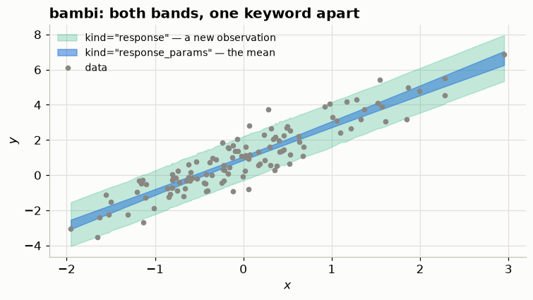

Predicting out of sample.

Hand predict a new dataframe and it does the rest — no pm.Data, no set_data, no rebuilding the model.

# Deliberately extrapolate beyond the observed range of x.
new_x = pd.DataFrame({"x": np.linspace(data["x"].min() - 2, data["x"].max() + 2, 60)})
oos = model_bmb.predict(idata_bmb, kind="response", data=new_x, inplace=False)

pp_new = oos["posterior_predictive"].dataset["y"].values
pp_new = pp_new.reshape(-1, pp_new.shape[-1])
lo_n, mid_n, hi_n = np.percentile(pp_new, [5.5, 50, 94.5], axis=0)

fig, ax = plt.subplots(figsize=(7, 4))
ax.axvspan(data["x"].min(), data["x"].max(), color=S.MUTED, alpha=0.12,
           label="range of observed $x$")
ax.fill_between(new_x["x"], lo_n, hi_n, color=S.ALT, alpha=0.22,
                label="89% predictive, new $x$")
ax.plot(new_x["x"], mid_n, color=S.ALT, lw=2, label="predictive median")
ax.plot(data["x"], data["y"], "o", color=S.MUTED, ms=4, ls="none", label="data")
ax.set(title="Conditioning on covariates the model never saw",
       xlabel="$x$", ylabel="$y$")
ax.legend(fontsize=9)
fig.tight_layout()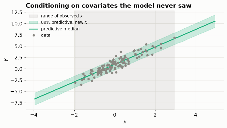

💡 This is the argument for bambi in one picture

model.predict(idata, data=new_x) — that is the whole out-of-sample story. For any model whose structure bambi can express, you get prediction, marginalisation over covariates, and the bmb.interpret tools (predictions, comparisons, slopes) without writing them.

Note the band widens outside the shaded region. The model is extrapolating, and it says so. It is still only honest about the uncertainty it knows about — a straight line assumed to keep being straight. Widening error bars are not a warrant for trusting an extrapolation.

Transfer Learning

bambi is a front end, not a different engine. Everything you learn about PyMC sampling, diagnostics and DataTree applies unchanged — which is why we did it in this order.

Exercise 3

Add a grouping variable to the simulated data (say 5 groups with different intercepts), then write the bambi formula for a model with a random intercept per group. Fit it and check that the group-level parameters appear in the posterior. (Note the Wilkinson notation for the random intercept: “({effect} | {grouping_variable})”)

Solution

g = rng.integers(0, 5, n)
offsets = rng.normal(0, 1.5, 5)
data2 = data.assign(group=[f"g{i}" for i in g],
                    y=data["y"] + offsets[g])

m = bmb.Model("y ~ x + (1|group)", data2)
print(m)
idata2 = m.fit(draws=1000, tune=1000, chains=4, cores=1,
               progressbar=False, random_seed=RANDOM_SEED)
print(az.summary(idata2, kind="stats").to_string())

(1|group) is a random intercept. You should see 1|group entries plus a 1|group_sigma — the population spread of the group intercepts. That _sigma is the parameter whose geometry we spend all of Day 3, 11:00 on.

6. Optional: the `do` operator

(Skip if we are short on time — nothing later depends on it. But it is the mechanism behind every “dataset whose truth we know” in this course, so it is worth ten minutes at some point.)

PyMC can intervene on a model, not just condition on it. pm.do replaces a variable with a fixed value and cuts the arrows coming into it. That is a different operation from observing the same value, and the difference is the whole of causal inference in one idea.

It has a second use that matters more for us day to day, and we come back to it at the end of this section: do is how you turn a fitted model back into a generator with parameters you choose, which is exactly what a parameter recovery study needs.

To see it you need a model where something upstream exists. Take a chain:

\[ z \sim \text{Normal}(0, 1), \qquad x \mid z \sim \text{Normal}(z,\ 0.5), \qquad y \mid x \sim \text{Normal}(x,\ 0.5). \]

Now ask what we learn about \(z\) in two scenarios: we observe \(x = 2\), versus we set \(x = 2\) ourselves.

with pm.Model() as chain:
    z = pm.Normal("z", 0.0, 1.0)
    x_var = pm.Normal("x_var", mu=z, sigma=0.5)
    pm.Normal("y_var", mu=x_var, sigma=0.5)

# Both functions return a NEW model; `chain` itself is untouched.
observed = pm.observe(chain, {chain["x_var"]: 2.0})    # condition
intervened = pm.do(chain, {chain["x_var"]: 2.0})       # intervene

Look at what each one did to the graph

This is the clearest way to see the difference, and it is structural rather than statistical — you can read the answer off the picture before running a single sampler.

from IPython.display import HTML, display


def _graph_svg(model):
    return pm.model_to_graphviz(model).pipe(format="svg").decode()


try:
    display(HTML(
        '<div style="display:flex; gap:3rem; align-items:flex-start; '
        'flex-wrap:wrap">'
        f'<div><b>original model</b><br>{_graph_svg(chain)}</div>'
        f'<div><b>pm.observe(x_var = 2)</b><br>{_graph_svg(observed)}</div>'
        f'<div><b>pm.do(x_var = 2)</b><br>{_graph_svg(intervened)}</div>'
        '</div>'))
except Exception as exc:                      # graphviz needs the `dot` BINARY
    print(f"graphviz unavailable ({type(exc).__name__}); mermaid instead\n")
    for name, m in [("ORIGINAL", chain), ("OBSERVE", observed), ("DO", intervened)]:
        print(f"--- {name} ---")
        print(pm.model_to_mermaid(m), "\n")

original model

pm.observe(x_var = 2)

pm.do(x_var = 2)

Read the three graphs left to right:

Original. z → x_var → y_var, all three open (unobserved).
pm.observe. x_var is now shaded — it is data. But the arrow z → x_var is still there. That edge is the channel evidence travels along, and it runs in both directions: knowing x_var tells you about z.
pm.do. x_var is no longer a random variable at all; it has become a constant, and the arrow from z is gone. z is now disconnected from everything downstream.

That missing arrow is the entire content of the do-operator. Once it is cut, no amount of sampling can send information from x_var back to z — not because we told it not to, but because there is no path.

Now confirm that the graphs predicted the numbers:

# (a) OBSERVE x = 2  -> evidence flows backwards along the surviving edge
with observed:
    idata_obs = pm.sample(draws=1000, tune=1000, chains=2, cores=1,
                          nuts_sampler="pymc", progressbar=False,
                          random_seed=RANDOM_SEED)

# (b) DO x = 2  -> the z -> x arrow is cut, so z keeps its prior
with intervened:
    idata_do = pm.sample_prior_predictive(draws=2000, random_seed=RANDOM_SEED)

z_obs = idata_obs.posterior.dataset["z"].values.ravel()
z_do = idata_do["prior"].dataset["z"].values.ravel()
print(f"E[z | observe x=2] = {z_obs.mean():+.3f}")
print(f"E[z | do(x=2)]     = {z_do.mean():+.3f}   (prior mean is 0)")

Initializing NUTS using jitter+adapt_diag...
Sequential sampling (2 chains in 1 job)
NUTS: [z, y_var]
Sampling 2 chains for 1_000 tune and 1_000 draw iterations (2_000 + 2_000 draws total) took 0 seconds.
We recommend running at least 4 chains for robust computation of convergence diagnostics
Sampling: [y_var, z]

E[z | observe x=2] = +1.582
E[z | do(x=2)]     = +0.004   (prior mean is 0)

fig, ax = plt.subplots(figsize=(7, 3.8))
bins = np.linspace(-3.5, 3.5, 70)
ax.hist(z_do, bins=bins, density=True, color=S.NAIVE, alpha=0.65,
        label="$do(x=2)$ — intervene")
ax.hist(z_obs, bins=bins, density=True, color=S.PRIMARY, alpha=0.75,
        label="observe $x=2$ — condition")
S.truth_line(ax, 0.0, axis="x", label="prior mean of $z$")
ax.set(title="Observing is not intervening", xlabel="$z$", ylabel="density")
ax.legend()
fig.tight_layout()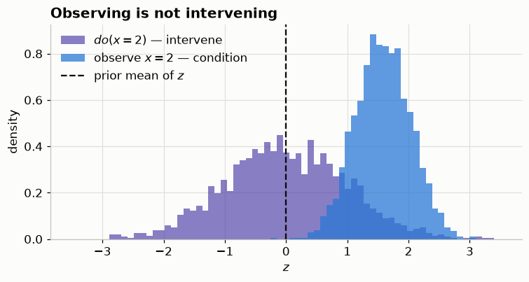

Observing \(x = 2\) is evidence: \(x\) is downstream of \(z\), so a high \(x\) makes a high \(z\) more plausible and the posterior shifts. Intervening — reaching in and setting \(x\) — destroys that inferential link, because the value no longer came from \(z\). \(z\) keeps its prior.

📝 Why a modelling library has this at all

Once you can express interventions, a fitted model can answer “what would happen if we changed this?” rather than only “what tends to go with what?”. pm.do and pm.observe return new models, leaving the original untouched, so you can ask several such questions off one fit. HSSM exposes the same idea as model.sample_do(...) — you will see it on Day 3.

The use you will actually reach for: parameter recovery

Causal language aside, here is the everyday reason a cognitive modeller wants pm.do. A model you can fit is also a model you can generate from — and do is the switch between the two.

Pin every free parameter to a value you chose, draw from what remains, and you have a dataset whose true parameters you know exactly. Fit that dataset with the same model and you can ask the only question that really validates an analysis pipeline:

If the data really did come from this model, would I get the right answer back?

This is parameter recovery, and it is worth doing before any real dataset is touched. It catches an unidentifiable design, a coding error, a prior that is quietly doing the work, and a sampler that has not converged — none of which announce themselves on real data, where you never learn the truth.

The whole loop, on the model from section 2:

# 1. GENERATE — intervene on the model to fix mu and sigma at chosen values.
TRUE_PARAMS = {"mu": 4.2, "sigma": 0.8}

with pm.Model() as recovery_model:
    mu_r = pm.Normal("mu", 0.0, 10.0)
    sigma_r = pm.HalfNormal("sigma", 5.0)
    pm.Normal("y", mu=mu_r, sigma=sigma_r, shape=200)

generator = pm.do(recovery_model,
                  {recovery_model["mu"]: TRUE_PARAMS["mu"],
                   recovery_model["sigma"]: TRUE_PARAMS["sigma"]})
with generator:
    synthetic = pm.sample_prior_predictive(draws=1, random_seed=RANDOM_SEED)
y_synth = synthetic["prior"].dataset["y"].values.ravel()

print(f"generated {y_synth.size} observations "
      f"| sample mean {y_synth.mean():.3f}, sample sd {y_synth.std():.3f}")

Sampling: [y]

generated 200 observations | sample mean 4.207, sample sd 0.726

# 2. RECOVER — hand the synthetic data back to the SAME model and fit it.
with pm.Model() as fit_model:
    mu_f = pm.Normal("mu", 0.0, 10.0)
    sigma_f = pm.HalfNormal("sigma", 5.0)
    pm.Normal("y", mu=mu_f, sigma=sigma_f, observed=y_synth)
    idata_rec = pm.sample(draws=1000, tune=1000, chains=4, cores=1,
                          nuts_sampler="pymc", progressbar=False,
                          random_seed=RANDOM_SEED)

# 3. CHECK — does the posterior cover the values we generated with?
print(az.summary(idata_rec, kind="stats", ci_prob=0.89).to_string(), "\n")

# Compute the interval from the DRAWS, not by reading it back out of the
# summary table: az.summary returns formatted STRINGS rounded to a couple of
# significant figures, so `4.2` comes back as the string "4".
post_rec = idata_rec.posterior.dataset
for name, truth in TRUE_PARAMS.items():
    lo, hi = np.percentile(post_rec[name].values, [5.5, 94.5])
    print(f"  {name:6s} true {truth:5.2f}   89% interval [{lo:5.2f}, {hi:5.2f}]   "
          f"{'COVERED' if lo <= truth <= hi else '*** MISSED ***'}")

Initializing NUTS using jitter+adapt_diag...
Sequential sampling (4 chains in 1 job)
NUTS: [mu, sigma]
Sampling 4 chains for 1_000 tune and 1_000 draw iterations (4_000 + 4_000 draws total) took 0 seconds.

       mean     sd eti89_lb eti89_ub
mu      4.2  0.054      4.1      4.3
sigma  0.73  0.037     0.68     0.79 

  mu     true  4.20   89% interval [ 4.12,  4.29]   COVERED
  sigma  true  0.80   89% interval [ 0.68,  0.79]   *** MISSED ***

Look closely at that result before drawing a conclusion from it: mu is covered and sigma is not — its 89% interval stops just short of 0.80.

Nothing is broken. The 200 numbers we generated happen to have a sample sd of about 0.73, and the posterior has correctly recovered the data it was given. With \(n = 200\) the sampling sd of a sample sd is roughly \(\sigma/\sqrt{2n} \approx 0.04\), so landing 0.07 low is an ordinary draw.

Which exposes the real lesson: one recovery run tells you almost nothing. An 89% interval is supposed to miss about 11% of the time. A single run that covers is weak evidence, and a single run that misses is not a bug report.

The honest version repeats the whole loop over many simulated datasets and asks whether the intervals cover at their nominal rate:

def recover_once(seed, n=200):
    """Generate one dataset from TRUE_PARAMS, refit, return the 89% intervals."""
    with pm.Model() as gen:
        pm.Normal("mu", 0.0, 10.0)
        pm.HalfNormal("sigma", 5.0)
        pm.Normal("y", mu=gen["mu"], sigma=gen["sigma"], shape=n)

    with pm.do(gen, {gen["mu"]: TRUE_PARAMS["mu"],
                     gen["sigma"]: TRUE_PARAMS["sigma"]}):
        ys = (pm.sample_prior_predictive(draws=1, random_seed=seed)
              ["prior"].dataset["y"].values.ravel())

    with pm.Model() as fit:
        pm.Normal("mu", 0.0, 10.0)
        pm.HalfNormal("sigma", 5.0)
        pm.Normal("y", mu=fit["mu"], sigma=fit["sigma"], observed=ys)
        idt = pm.sample(600, tune=600, chains=2, cores=1, nuts_sampler="pymc",
                        progressbar=False, random_seed=seed)

    return {k: np.percentile(idt.posterior.dataset[k].values, [5.5, 94.5])
            for k in TRUE_PARAMS}


N_REPS = 40
hits = {k: 0 for k in TRUE_PARAMS}
for seed in range(N_REPS):
    for k, (lo, hi) in recover_once(seed).items():
        hits[k] += lo <= TRUE_PARAMS[k] <= hi

print(f"{N_REPS} simulated datasets, 89% intervals:\n")
for k, n_hit in hits.items():
    print(f"  {k:6s} covered {n_hit:2d}/{N_REPS} = {n_hit / N_REPS:.0%}   "
          f"(nominal 89%)")

Sampling: [y]
Initializing NUTS using jitter+adapt_diag...
Sequential sampling (2 chains in 1 job)
NUTS: [mu, sigma]
Sampling 2 chains for 600 tune and 600 draw iterations (1_200 + 1_200 draws total) took 0 seconds.
We recommend running at least 4 chains for robust computation of convergence diagnostics
The rhat statistic is larger than 1.01 for some parameters. This indicates problems during sampling. See https://arxiv.org/abs/1903.08008 for details
Sampling: [y]
Initializing NUTS using jitter+adapt_diag...
Sequential sampling (2 chains in 1 job)
NUTS: [mu, sigma]
Sampling 2 chains for 600 tune and 600 draw iterations (1_200 + 1_200 draws total) took 0 seconds.
We recommend running at least 4 chains for robust computation of convergence diagnostics
Sampling: [y]
Initializing NUTS using jitter+adapt_diag...
Sequential sampling (2 chains in 1 job)
NUTS: [mu, sigma]
Sampling 2 chains for 600 tune and 600 draw iterations (1_200 + 1_200 draws total) took 0 seconds.
We recommend running at least 4 chains for robust computation of convergence diagnostics
Sampling: [y]
Initializing NUTS using jitter+adapt_diag...
Sequential sampling (2 chains in 1 job)
NUTS: [mu, sigma]
Sampling 2 chains for 600 tune and 600 draw iterations (1_200 + 1_200 draws total) took 0 seconds.
We recommend running at least 4 chains for robust computation of convergence diagnostics
Sampling: [y]
Initializing NUTS using jitter+adapt_diag...
Sequential sampling (2 chains in 1 job)
NUTS: [mu, sigma]
Sampling 2 chains for 600 tune and 600 draw iterations (1_200 + 1_200 draws total) took 0 seconds.
We recommend running at least 4 chains for robust computation of convergence diagnostics
Sampling: [y]
Initializing NUTS using jitter+adapt_diag...
Sequential sampling (2 chains in 1 job)
NUTS: [mu, sigma]
Sampling 2 chains for 600 tune and 600 draw iterations (1_200 + 1_200 draws total) took 0 seconds.
We recommend running at least 4 chains for robust computation of convergence diagnostics
Sampling: [y]
Initializing NUTS using jitter+adapt_diag...
Sequential sampling (2 chains in 1 job)
NUTS: [mu, sigma]
Sampling 2 chains for 600 tune and 600 draw iterations (1_200 + 1_200 draws total) took 0 seconds.
We recommend running at least 4 chains for robust computation of convergence diagnostics
Sampling: [y]
Initializing NUTS using jitter+adapt_diag...
Sequential sampling (2 chains in 1 job)
NUTS: [mu, sigma]
Sampling 2 chains for 600 tune and 600 draw iterations (1_200 + 1_200 draws total) took 0 seconds.
We recommend running at least 4 chains for robust computation of convergence diagnostics
Sampling: [y]
Initializing NUTS using jitter+adapt_diag...
Sequential sampling (2 chains in 1 job)
NUTS: [mu, sigma]
Sampling 2 chains for 600 tune and 600 draw iterations (1_200 + 1_200 draws total) took 0 seconds.
We recommend running at least 4 chains for robust computation of convergence diagnostics
Sampling: [y]
Initializing NUTS using jitter+adapt_diag...
Sequential sampling (2 chains in 1 job)
NUTS: [mu, sigma]
Sampling 2 chains for 600 tune and 600 draw iterations (1_200 + 1_200 draws total) took 0 seconds.
We recommend running at least 4 chains for robust computation of convergence diagnostics
Sampling: [y]
Initializing NUTS using jitter+adapt_diag...
Sequential sampling (2 chains in 1 job)
NUTS: [mu, sigma]
Sampling 2 chains for 600 tune and 600 draw iterations (1_200 + 1_200 draws total) took 0 seconds.
We recommend running at least 4 chains for robust computation of convergence diagnostics
Sampling: [y]
Initializing NUTS using jitter+adapt_diag...
Sequential sampling (2 chains in 1 job)
NUTS: [mu, sigma]
Sampling 2 chains for 600 tune and 600 draw iterations (1_200 + 1_200 draws total) took 0 seconds.
We recommend running at least 4 chains for robust computation of convergence diagnostics
Sampling: [y]
Initializing NUTS using jitter+adapt_diag...
Sequential sampling (2 chains in 1 job)
NUTS: [mu, sigma]
Sampling 2 chains for 600 tune and 600 draw iterations (1_200 + 1_200 draws total) took 0 seconds.
We recommend running at least 4 chains for robust computation of convergence diagnostics
Sampling: [y]
Initializing NUTS using jitter+adapt_diag...
Sequential sampling (2 chains in 1 job)
NUTS: [mu, sigma]
Sampling 2 chains for 600 tune and 600 draw iterations (1_200 + 1_200 draws total) took 0 seconds.
We recommend running at least 4 chains for robust computation of convergence diagnostics
Sampling: [y]
Initializing NUTS using jitter+adapt_diag...
Sequential sampling (2 chains in 1 job)
NUTS: [mu, sigma]
Sampling 2 chains for 600 tune and 600 draw iterations (1_200 + 1_200 draws total) took 0 seconds.
We recommend running at least 4 chains for robust computation of convergence diagnostics
Sampling: [y]
Initializing NUTS using jitter+adapt_diag...
Sequential sampling (2 chains in 1 job)
NUTS: [mu, sigma]
Sampling 2 chains for 600 tune and 600 draw iterations (1_200 + 1_200 draws total) took 0 seconds.
We recommend running at least 4 chains for robust computation of convergence diagnostics
Sampling: [y]
Initializing NUTS using jitter+adapt_diag...
Sequential sampling (2 chains in 1 job)
NUTS: [mu, sigma]
Sampling 2 chains for 600 tune and 600 draw iterations (1_200 + 1_200 draws total) took 0 seconds.
We recommend running at least 4 chains for robust computation of convergence diagnostics
Sampling: [y]
Initializing NUTS using jitter+adapt_diag...
Sequential sampling (2 chains in 1 job)
NUTS: [mu, sigma]
Sampling 2 chains for 600 tune and 600 draw iterations (1_200 + 1_200 draws total) took 0 seconds.
We recommend running at least 4 chains for robust computation of convergence diagnostics
Sampling: [y]
Initializing NUTS using jitter+adapt_diag...
Sequential sampling (2 chains in 1 job)
NUTS: [mu, sigma]
Sampling 2 chains for 600 tune and 600 draw iterations (1_200 + 1_200 draws total) took 0 seconds.
We recommend running at least 4 chains for robust computation of convergence diagnostics
Sampling: [y]
Initializing NUTS using jitter+adapt_diag...
Sequential sampling (2 chains in 1 job)
NUTS: [mu, sigma]
Sampling 2 chains for 600 tune and 600 draw iterations (1_200 + 1_200 draws total) took 0 seconds.
We recommend running at least 4 chains for robust computation of convergence diagnostics
Sampling: [y]
Initializing NUTS using jitter+adapt_diag...
Sequential sampling (2 chains in 1 job)
NUTS: [mu, sigma]
Sampling 2 chains for 600 tune and 600 draw iterations (1_200 + 1_200 draws total) took 0 seconds.
We recommend running at least 4 chains for robust computation of convergence diagnostics
Sampling: [y]
Initializing NUTS using jitter+adapt_diag...
Sequential sampling (2 chains in 1 job)
NUTS: [mu, sigma]
Sampling 2 chains for 600 tune and 600 draw iterations (1_200 + 1_200 draws total) took 0 seconds.
We recommend running at least 4 chains for robust computation of convergence diagnostics
Sampling: [y]
Initializing NUTS using jitter+adapt_diag...
Sequential sampling (2 chains in 1 job)
NUTS: [mu, sigma]
Sampling 2 chains for 600 tune and 600 draw iterations (1_200 + 1_200 draws total) took 0 seconds.
We recommend running at least 4 chains for robust computation of convergence diagnostics
Sampling: [y]
Initializing NUTS using jitter+adapt_diag...
Sequential sampling (2 chains in 1 job)
NUTS: [mu, sigma]
Sampling 2 chains for 600 tune and 600 draw iterations (1_200 + 1_200 draws total) took 0 seconds.
We recommend running at least 4 chains for robust computation of convergence diagnostics
Sampling: [y]
Initializing NUTS using jitter+adapt_diag...
Sequential sampling (2 chains in 1 job)
NUTS: [mu, sigma]
Sampling 2 chains for 600 tune and 600 draw iterations (1_200 + 1_200 draws total) took 0 seconds.
We recommend running at least 4 chains for robust computation of convergence diagnostics
Sampling: [y]
Initializing NUTS using jitter+adapt_diag...
Sequential sampling (2 chains in 1 job)
NUTS: [mu, sigma]
Sampling 2 chains for 600 tune and 600 draw iterations (1_200 + 1_200 draws total) took 0 seconds.
We recommend running at least 4 chains for robust computation of convergence diagnostics
Sampling: [y]
Initializing NUTS using jitter+adapt_diag...
Sequential sampling (2 chains in 1 job)
NUTS: [mu, sigma]
Sampling 2 chains for 600 tune and 600 draw iterations (1_200 + 1_200 draws total) took 0 seconds.
We recommend running at least 4 chains for robust computation of convergence diagnostics
Sampling: [y]
Initializing NUTS using jitter+adapt_diag...
Sequential sampling (2 chains in 1 job)
NUTS: [mu, sigma]
Sampling 2 chains for 600 tune and 600 draw iterations (1_200 + 1_200 draws total) took 0 seconds.
We recommend running at least 4 chains for robust computation of convergence diagnostics
Sampling: [y]
Initializing NUTS using jitter+adapt_diag...
Sequential sampling (2 chains in 1 job)
NUTS: [mu, sigma]
Sampling 2 chains for 600 tune and 600 draw iterations (1_200 + 1_200 draws total) took 0 seconds.
We recommend running at least 4 chains for robust computation of convergence diagnostics
Sampling: [y]
Initializing NUTS using jitter+adapt_diag...
Sequential sampling (2 chains in 1 job)
NUTS: [mu, sigma]
Sampling 2 chains for 600 tune and 600 draw iterations (1_200 + 1_200 draws total) took 0 seconds.
We recommend running at least 4 chains for robust computation of convergence diagnostics
Sampling: [y]
Initializing NUTS using jitter+adapt_diag...
Sequential sampling (2 chains in 1 job)
NUTS: [mu, sigma]
Sampling 2 chains for 600 tune and 600 draw iterations (1_200 + 1_200 draws total) took 0 seconds.
We recommend running at least 4 chains for robust computation of convergence diagnostics
Sampling: [y]
Initializing NUTS using jitter+adapt_diag...
Sequential sampling (2 chains in 1 job)
NUTS: [mu, sigma]
Sampling 2 chains for 600 tune and 600 draw iterations (1_200 + 1_200 draws total) took 0 seconds.
We recommend running at least 4 chains for robust computation of convergence diagnostics
Sampling: [y]
Initializing NUTS using jitter+adapt_diag...
Sequential sampling (2 chains in 1 job)
NUTS: [mu, sigma]
Sampling 2 chains for 600 tune and 600 draw iterations (1_200 + 1_200 draws total) took 0 seconds.
We recommend running at least 4 chains for robust computation of convergence diagnostics
Sampling: [y]
Initializing NUTS using jitter+adapt_diag...
Sequential sampling (2 chains in 1 job)
NUTS: [mu, sigma]
Sampling 2 chains for 600 tune and 600 draw iterations (1_200 + 1_200 draws total) took 0 seconds.
We recommend running at least 4 chains for robust computation of convergence diagnostics
Sampling: [y]
Initializing NUTS using jitter+adapt_diag...
Sequential sampling (2 chains in 1 job)
NUTS: [mu, sigma]
Sampling 2 chains for 600 tune and 600 draw iterations (1_200 + 1_200 draws total) took 0 seconds.
We recommend running at least 4 chains for robust computation of convergence diagnostics
Sampling: [y]
Initializing NUTS using jitter+adapt_diag...
Sequential sampling (2 chains in 1 job)
NUTS: [mu, sigma]
Sampling 2 chains for 600 tune and 600 draw iterations (1_200 + 1_200 draws total) took 0 seconds.
We recommend running at least 4 chains for robust computation of convergence diagnostics
Sampling: [y]
Initializing NUTS using jitter+adapt_diag...
Sequential sampling (2 chains in 1 job)
NUTS: [mu, sigma]
Sampling 2 chains for 600 tune and 600 draw iterations (1_200 + 1_200 draws total) took 0 seconds.
We recommend running at least 4 chains for robust computation of convergence diagnostics
Sampling: [y]
Initializing NUTS using jitter+adapt_diag...
Sequential sampling (2 chains in 1 job)
NUTS: [mu, sigma]
Sampling 2 chains for 600 tune and 600 draw iterations (1_200 + 1_200 draws total) took 0 seconds.
We recommend running at least 4 chains for robust computation of convergence diagnostics
Sampling: [y]
Initializing NUTS using jitter+adapt_diag...
Sequential sampling (2 chains in 1 job)
NUTS: [mu, sigma]
Sampling 2 chains for 600 tune and 600 draw iterations (1_200 + 1_200 draws total) took 0 seconds.
We recommend running at least 4 chains for robust computation of convergence diagnostics
Sampling: [y]
Initializing NUTS using jitter+adapt_diag...
Sequential sampling (2 chains in 1 job)
NUTS: [mu, sigma]
Sampling 2 chains for 600 tune and 600 draw iterations (1_200 + 1_200 draws total) took 0 seconds.
We recommend running at least 4 chains for robust computation of convergence diagnostics

40 simulated datasets, 89% intervals:

  mu     covered 35/40 = 88%   (nominal 89%)
  sigma  covered 38/40 = 95%   (nominal 89%)

Both land near 89%, which is the result you want: the intervals are calibrated. Had one come back at 60%, the model would be overconfident and no single fit from it could be trusted — and you would never have found that out from one run, or from any amount of real data.

📝 Read the coverage numbers with their own error bars

With 40 replications, the standard error on a coverage estimate near 0.89 is about \(\sqrt{0.89 \times 0.11 / 40} \approx 5\%\). So anything from roughly 79% to 99% is consistent with a correctly calibrated interval, and you should not read a difference of one or two hits as a finding. Serious calibration work uses hundreds of replications — or simulation-based calibration, which checks the whole rank distribution rather than one interval, and which this summer school covers in its own right.

Note what pm.do bought us: one model definition served as both the generator and the estimator. Without it you would write the simulation twice — once as numpy, once as a PyMC model — and the two versions drift apart. The bug that then survives is the worst kind, because your recovery study is validating the wrong thing and passing.

💡 Where this goes for cognitive models

Everything above generalises directly, and the rest of the course leans on it:

At 14:30 today you fit a DDM to data simulated from known parameters, and check recovery cell by cell. At 15:00 you meet a design where recovery fails — drift and non-decision time trade off — and the only reason you can tell is that the truth is known.
Tomorrow at 09:30, HSSM’s model.sample_do(...) is this exact operation with a nicer signature: pin v, a, z, t (or the coefficients of a regression on them) and draw a dataset. The DDM dataset in that session is built precisely this way.
For a real study, run recovery across a grid of plausible parameters rather than one point. A model can recover beautifully at the centre of parameter space and fall apart at the edges, and the edge is often where your participants are.

The habit to take away: before fitting a new model to real data, fit it to fake data from itself. It is cheap, and it is the only setting in which you ever get to grade your own answer.

What to take away

💡 The things that matter

A distribution is used two ways. pm.Normal.dist(...) is a value you can draw from and take logp of. pm.Normal("name", ...) inside a model context is a node in a graph, and the name is how you get results back.
You are building a graph, behind the scenes. PyTensor allows you to compile the graph into multiple backend frameworks.
Bambi is a front-end to PyMC that makes specifying hierarchical mixed-effects regressions much easier. It is, in turn, the primary backend for HSSM.
Name your dimensions. coords + dims cost one dictionary and give you mu[high] instead of mu[2], everywhere downstream — including in the labels HSSM hands back tomorrow.
pm.do turns a model into its own data generator. Pin the parameters, simulate, refit, check the truth is covered. Do this before any real data.

Next: We stop assuming the sampler works, and start looking at when it does not.

Where PyMC comes from, and what it actually does

A very short history

The idea it shares with deep learning frameworks

The neighbourhood

1. What is a PyMC distribution?

Standalone

Densities, not just draws

Distributions inside a PyMC model

2. A first model, and what pm.sample() returns

Look at the model before you look at the answer

Data Structures that can cause confusion

What you get once you are on the Dataset

coords and dims — naming your own dimensions

3. Looking at a posterior

What conditioning on data actually did

Exercise 1

Exercise 2

4. A regression, by hand

Two bands that are not the same thing

Why the wide band looks like it has constant width

5. The same regression, in bambi

There is no magic — look at the generated model

Where bambi actually earns its keep

Predicting out of sample.

Transfer Learning

Exercise 3

6. Optional: the do operator

Look at what each one did to the graph

The use you will actually reach for: parameter recovery

What to take away

2. A first model, and what `pm.sample()` returns

What you get once you are on the `Dataset`

`coords` and `dims` — naming your own dimensions

6. Optional: the `do` operator