# --- Google Colab bootstrap; does nothing anywhere else ---------------------
import importlib.util, subprocess, sys, urllib.error, urllib.request

IN_COLAB = importlib.util.find_spec("google.colab") is not None

# `main` once this is merged; the branch is the fallback so the Colab path can
# be tested BEFORE the merge, when main does not yet have these files.
_REFS = ("main", "afengler.tutorials")
_RAW = "https://raw.githubusercontent.com/stefanradev93/sbi4cogsci/{ref}/tutorials/"


def _fetch(module):
    for ref in _REFS:
        try:
            urllib.request.urlretrieve(_RAW.format(ref=ref) + module, module)
            return ref
        except urllib.error.HTTPError:
            continue
    raise RuntimeError(f"could not fetch {module} from any of {_REFS}")


if IN_COLAB:
    # numba>=0.61 is REQUIRED, not cosmetic. pytensor resolves linker="auto" to
    # its numba backend, and numba renamed FunctionModel's first field
    # addr -> c_addr in 0.61. Colab preinstalls an older numba, and pytensor
    # declares numba only as an optional extra, so pip leaves it in place and
    # any MvNormal (SolveTriangular has no C implementation) dies with
    # KeyError: "FunctionModel does not have a field named 'c_addr'".
    subprocess.run([sys.executable, "-m", "pip", "install", "-q",
                    "numba>=0.61", "pymc>=6.2", "arviz>=1.2", "hssm>=0.4"],
                   check=True)
    for _mod in ["sbi4cogsci_style.py"]:
        print(f"  fetched {_mod} from {_fetch(_mod)}")
print("Colab setup done.")MCMC methods, and when inference falls apart
Day 2, 15:00 — 30 minutes. Alexander Fengler.
Everything you fitted this morning and at 14:30 converged quietly. That is not guaranteed, and the failures teach more than the successes. This session has two halves:
- what MCMC is actually doing — including writing a sampler from scratch in ten lines, so it stops being a black box;
- what makes a posterior hard, on the cognitive model you just fitted.
One idea runs through both. A posterior can be hard because of its shape, and past a certain point no amount of sampler tuning repairs a bad shape — you have to change the sampler, or change the experiment.
▶️ Running this on Google Colab
The cell below is a no-op on your own machine. On Colab it installs the stack and downloads the shared helper module, which lives one directory up in the repository and is therefore not importable there.
Expect the install to take a few minutes. If Colab asks you to restart the runtime, do it and then run the cell again — the second run is a no-op.
import sys, pathlib, warnings, time
sys.path.insert(0, str(pathlib.Path.cwd().parent))  # -> tutorials/

import numpy as np
import pandas as pd
import matplotlib.pyplot as plt
import pymc as pm
import arviz as az
import sbi4cogsci_style as S

S.use()
warnings.filterwarnings("ignore")

RANDOM_SEED = sum(map(ord, "sbi4cogsci-mcmc"))
rng = np.random.default_rng(RANDOM_SEED)

print("pymc", pm.__version__, "| arviz", az.__version__)
pymc 6.2.0 | arviz 1.2.01. What is MCMC actually trying to do?
Everything you want from a posterior — a mean, a credible interval, a posterior predictive — is an integral against it, and in more than two or three dimensions those integrals are hopeless. So we stop computing them and draw samples instead, then average.
Which leaves one obstacle. Bayes’ rule gives the posterior as \(p(y \mid \theta)\,p(\theta) / p(y)\), and that denominator — the evidence — is itself an integral over the whole parameter space, exactly the thing we just admitted we cannot do.
The escape is that every MCMC algorithm only ever looks at ratios. Writing the unnormalised density as \(\tilde{\pi} = p(y \mid \theta)p(\theta)\),
\[ \frac{\pi(\theta')}{\pi(\theta)} \;=\; \frac{\tilde{\pi}(\theta') / p(y)}{\tilde{\pi}(\theta) / p(y)} \;=\; \frac{\tilde{\pi}(\theta')}{\tilde{\pi}(\theta)} . \]
\(p(y)\) cancels, and you never need the evidence to sample a posterior — only to compare whole models against each other. (Nothing here mentions Bayes, incidentally: MCMC samples any distribution you can evaluate up to a constant.)
2. A Metropolis sampler in ten lines
The oldest MCMC algorithm, and still the clearest. From the current point \(\theta\):
- propose a nearby point, \(\theta' = \theta + \varepsilon\) with \(\varepsilon \sim \text{Normal}(0, s^2)\);
- accept it with probability \(\alpha = \min\!\left(1,\ \tilde{\pi}(\theta')/\tilde{\pi}(\theta)\right)\);
- if accepted move there, otherwise stay put and record the current point again.
Because the proposal is symmetric, that ratio is the whole rule. Step 3 is the part people find strange: rejecting does not mean discarding the iteration, it means the chain repeats itself — which is how low-density regions end up visited proportionally less, rather than never.
def metropolis(log_target, start, n_steps=100_000, step_size=1.0, seed=0):
    """Random-walk Metropolis. `log_target` need only be correct up to a constant."""
    rng = np.random.default_rng(seed)
    theta = np.atleast_1d(np.asarray(start, dtype=float))
    logp = log_target(theta)
    chain, n_accept = np.empty((n_steps, theta.size)), 0

    for i in range(n_steps):
        proposal = theta + rng.normal(0.0, step_size, theta.size)
        logp_prop = log_target(proposal)
        # accept with probability min(1, pi(prop)/pi(theta)) — in logs
        if np.log(rng.uniform()) < logp_prop - logp:
            theta, logp = proposal, logp_prop
            n_accept += 1
        chain[i] = theta

    return chain, n_accept / n_steps
To show that the normalizing constant genuinely does not matter, target a distribution written without one. This is a Gaussian mixture whose true density we happen to know, so we can check the answer:
def log_target_mixture(theta):
    """log of an UNNORMALISED two-component mixture. No 1/sqrt(2*pi) anywhere."""
    x = theta[0]
    return np.log(np.exp(-0.5 * ((x - 2.0) / 0.7) ** 2)
                  + 0.6 * np.exp(-0.5 * ((x + 1.5) / 0.5) ** 2))


chain, acc = metropolis(log_target_mixture, start=[0.0], step_size=1.5,
                        n_steps=100_000, seed=RANDOM_SEED)
print(f"acceptance rate {acc:.2f}")

grid = np.linspace(-4, 5, 400)
dens = np.exp([log_target_mixture([g]) for g in grid])
dens /= np.trapezoid(dens, grid)          # normalise only for PLOTTING

fig, ax = plt.subplots(figsize=(7, 3.8))
ax.hist(chain[2000:, 0], bins=90, density=True, color=S.PRIMARY, alpha=0.75,
        label="Metropolis samples")
ax.plot(grid, dens, color=S.TRUTH, ls="--", lw=2, label="true density")
ax.set(title="Sampling a distribution we never normalised",
       xlabel=r"$\theta$", ylabel="density")
ax.legend()
fig.tight_layout()
acceptance rate 0.51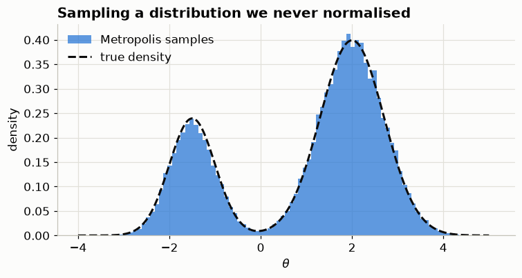
A dozen lines of Python, no gradients, no library — and the histogram lands on the density, without ever computing the normalizing constant.
Poll. Our proposal was symmetric: \(\theta' = \theta + \text{Normal}(0, s^2)\). What breaks if the proposal is asymmetric and we keep this same rule?
- A. Nothing — the chain still targets \(\pi\).
- B. The chain converges to the wrong distribution.
- C. The chain still works but mixes more slowly.
- D. The acceptance rate goes to zero.
Answer
B. With an asymmetric proposal you must include the proposal ratio too — the Metropolis–Hastings correction, \(\alpha = \min(1,\ [\tilde{\pi}(\theta')q(\theta \mid \theta')] / [\tilde{\pi}(\theta)q(\theta' \mid \theta)])\). Omit it and the chain converges happily to something that is not your target, with no warning. Our symmetric Gaussian proposal makes \(q\) cancel, which is why we could leave it out.
The same mixture, pulled apart
That worked because the two modes overlap: at \(\theta = 0\) the density is low but not negligible, so a chain crossing the valley is occasionally accepted. Push the modes apart and keep everything else identical, and the sampler stops working — completely, and quietly.
def log_target_split(theta):
    """The same two-component mixture, with the modes moved to -6 and +6."""
    x = theta[0]
    return np.log(np.exp(-0.5 * ((x - 6.0) / 0.6) ** 2)
                  + 0.6 * np.exp(-0.5 * ((x + 6.0) / 0.6) ** 2))


# Four chains, TWO started in each mode — the point is what each one does.
starts = [-6.0, -6.0, 6.0, 6.0]
split_chains = np.stack([
    metropolis(log_target_split, [s], n_steps=100_000, step_size=1.5,
               seed=RANDOM_SEED + i)[0][2_000:, 0]
    for i, s in enumerate(starts)])

for i, (s, ch) in enumerate(zip(starts, split_chains)):
    print(f"  chain {i} started at {s:+.0f}:  "
          f"{np.mean(ch > 0):.1%} of its draws in the RIGHT mode")

TRUE_RIGHT_WEIGHT = 1.0 / 1.6         # weights are 1.0 and 0.6
print(f"\npooled estimate of P(right mode) = {np.mean(split_chains > 0):.3f}"
      f"   (truth {TRUE_RIGHT_WEIGHT:.3f})")
chain 0 started at -6: 0.0% of its draws in the RIGHT mode
chain 1 started at -6: 0.0% of its draws in the RIGHT mode
chain 2 started at +6: 100.0% of its draws in the RIGHT mode
chain 3 started at +6: 100.0% of its draws in the RIGHT mode
pooled estimate of P(right mode) = 0.500 (truth 0.625)fig, axes = plt.subplots(1, 2, figsize=(11, 3.8),
gridspec_kw={"width_ratios": [1.4, 1]})
ax = axes[0]
for i, ch in enumerate(split_chains):
ax.plot(ch[:4000], lw=0.6, alpha=0.85,
color=S.PRIMARY if starts[i] > 0 else S.NAIVE)
ax.set(title="Four chains, and not one of them moves",
xlabel="draw", ylabel=r"$\theta$")
ax = axes[1]
grid_s = np.linspace(-9, 9, 500)
dens_s = np.exp([log_target_split([g]) for g in grid_s])
dens_s /= np.trapezoid(dens_s, grid_s)
ax.hist(split_chains.ravel(), bins=120, density=True, color=S.PRIMARY,
alpha=0.75, label="pooled samples")
ax.plot(grid_s, dens_s, color=S.TRUTH, ls="--", lw=2, label="true density")
ax.set(title="...so the weights come out wrong", xlabel=r"$\theta$",
ylabel="density")
ax.legend(fontsize=9)
fig.tight_layout()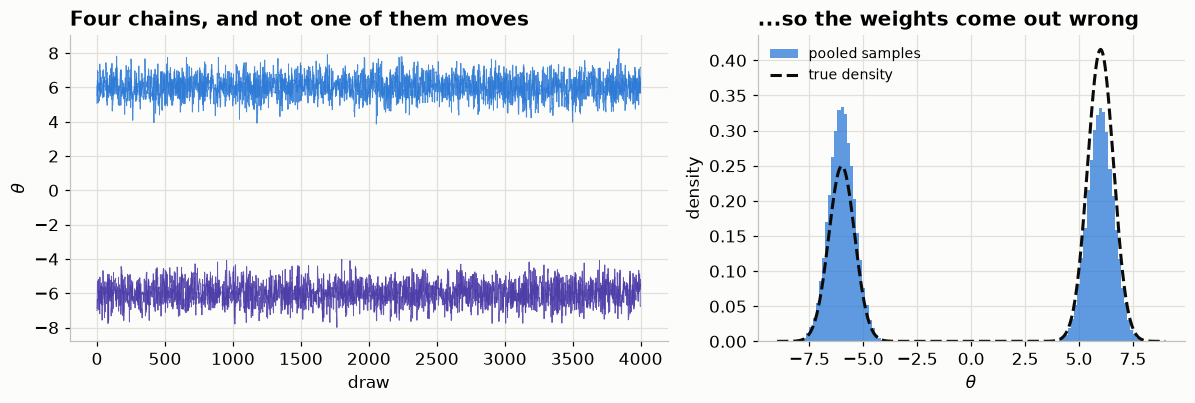
Every chain stays in the mode it started in for all 100,000 draws. Each one, on its own, looks perfectly healthy: it is stationary, it mixes briskly within its mode, and its acceptance rate is fine. Nothing in a single chain says “there is another mode over there.”
Pooling them does not rescue the answer either — it reports the two modes as equally likely, because we happened to start two chains in each, when the truth is 0.625 / 0.375. The estimate is an artifact of where we started.
dt_split = az.convert_to_datatree({"x": split_chains})
print(f"R-hat = {float(az.rhat(dt_split, var_names=['x']).x):.2f}"
      "     (want < 1.01)")
print(f"ESS   = {float(az.ess(dt_split, var_names=['x']).x):.1f}"
      f"      out of {split_chains.size:,} draws")
R-hat = 1.73 (want < 1.01)
ESS = 6.0 out of 392,000 draws🔑 R-hat only catches this because the chains disagree
\(\hat{R}\) compares the variance between chains to the variance within them. Here the between-chain variance is enormous, so it fires loudly.
But notice the precondition: we started the chains in different places. Run four chains from the same initial value and they would all find the same mode, agree with each other perfectly, and report \(\hat{R} \approx 1.00\) for an answer that is completely wrong. This is the single best argument for multiple chains from dispersed starting points, and it is why PyMC defaults to four chains with jittered initialisation rather than one.
Gradients do not save you here either. NUTS follows the geometry it is standing in, and there is no gradient path across a region of zero density — it is faster and better-behaved than what we wrote, and just as trapped. Genuinely multimodal posteriors need a different tool: tempering, nested sampling, or an explicitly enumerated mixture.
step_size is the whole art of a random-walk sampler. Too small and every proposal is accepted but the chain barely moves; too large and almost everything is rejected so the chain barely moves. Both failures look like “high” or “reasonable” acceptance rates.
rows = []
for s in [0.05, 0.5, 1.5, 5.0, 20.0]:
    ch, a = metropolis(log_target_mixture, start=[0.0], step_size=s,
                       n_steps=20_000, seed=RANDOM_SEED)
    x = ch[2000:, 0]
    ess = float(az.ess(az.convert_to_datatree({"x": x[None, :]}),
                       var_names=["x"]).x)
    rows.append({"step_size": s, "acceptance": a, "ESS": ess,
                 "ESS/draw": ess / x.size})
print(pd.DataFrame(rows).to_string(index=False, float_format=lambda v: f"{v:9.3f}"))
step_size acceptance ESS ESS/draw
0.050 0.970 56.313 0.003
0.500 0.757 71.015 0.004
1.500 0.505 1125.020 0.063
5.000 0.258 2437.447 0.135
20.000 0.072 818.132 0.045🔑 Acceptance rate is not a measure of quality
The smallest step size has by far the highest acceptance rate and among the worst ESS — it accepts everything because it proposes almost nothing. Judge a sampler by effective sample size, never by how often it says yes.
Notice what that table let us do: we tuned our way out of trouble. There was a bad setting and a good one, we found the good one, and the sampler worked. Hold on to that, because the next target takes it away.
3. When there is no good step size
The mixture was hard in an easy way: one knob, and a right answer for it. Now a target that is much simpler to write down and much harder to sample — a two-dimensional Gaussian with correlation \(\rho\):
\[ \log \tilde{\pi}(x_0, x_1) \;=\; -\,\frac{x_0^2 - 2\rho\, x_0 x_1 + x_1^2}{2\,(1 - \rho^2)} . \]
No multimodality, no heavy tails, no awkward constraint. Just an ellipse. As \(\rho \to 1\) that ellipse becomes a long thin ridge along the diagonal, and that alone is enough to defeat the sampler we just wrote.
def log_target_gaussian(rho):
    """Unnormalised 2-D Gaussian, unit marginals, correlation rho."""
    denom = 2.0 * (1.0 - rho**2)

    def log_target(theta):
        x0, x1 = theta[0], theta[1]
        return -(x0**2 - 2.0 * rho * x0 * x1 + x1**2) / denom

    return log_target


RHOS = [0.0, 0.9, 0.99]
for rho in RHOS:
    # the sd along each axis is sqrt(1 +/- rho)
    print(f"rho = {rho:4.2f}:  length {np.sqrt(1 + rho):.3f}   "
          f"width {np.sqrt(1 - rho):.3f}   "
          f"aspect ratio {np.sqrt((1 + rho) / (1 - rho)):6.2f} : 1")
rho = 0.00: length 1.000 width 1.000 aspect ratio 1.00 : 1
rho = 0.90: length 1.378 width 0.316 aspect ratio 4.36 : 1
rho = 0.99: length 1.411 width 0.100 aspect ratio 14.11 : 1At \(\rho = 0.99\) the target is fourteen times longer than it is wide. A random-walk proposal is a circle — the same size step in every direction — and no circle fits a shape like that.
Before measuring anything, watch it happen. Same sampler, same step size, same number of moves; only \(\rho\) changes.
def plot_path(ax, path, rho, title, alpha=0.1):
    """Chain path over the target's contours. Used for every sampler here.

    The path is drawn faint on purpose. Where the chain sits still, hundreds of
    overlapping segments stack up and the ink goes dark; where it moves freely,
    each segment is drawn once and stays pale. So darkness *is* the diagnostic:
    a black blob is a chain that stopped. The start marker stays opaque — it is
    a landmark, not part of the trace.
    """
    g = np.linspace(-3.5, 3.5, 200)
    X0, X1 = np.meshgrid(g, g)
    Z = np.exp(-(X0**2 - 2 * rho * X0 * X1 + X1**2) / (2 * (1 - rho**2)))
    ax.contour(X0, X1, Z, levels=5, colors=S.MUTED, linewidths=0.8)
    ax.plot(path[:, 0], path[:, 1], "-", color=S.NAIVE, lw=1.1, alpha=alpha)
    ax.plot(path[:, 0], path[:, 1], "o", color=S.NAIVE, ms=2.5, ls="none",
            alpha=min(1.0, alpha + 0.1))
    ax.plot(path[0, 0], path[0, 1], "o", color=S.DIVERGENT, ms=8, label="start")
    ax.set(title=title, xlabel="$x_0$", ylabel="$x_1$",
           xlim=(-3.5, 3.5), ylim=(-3.5, 3.5))


N_SHOW = 300
fig, axes = plt.subplots(1, 3, figsize=(13, 4.4), sharex=True, sharey=True)
for ax, rho in zip(axes, RHOS):
    path, _ = metropolis(log_target_gaussian(rho), start=[0.0, 0.0],
                         n_steps=N_SHOW, step_size=1.0, seed=RANDOM_SEED)
    ax.plot([], [])
    plot_path(ax, path, rho, rf"$\rho$ = {rho}")
axes[0].legend(fontsize=9, loc="upper left")
fig.suptitle(f"{N_SHOW} Metropolis moves, step size 1.0 throughout", y=1.02)
fig.tight_layout()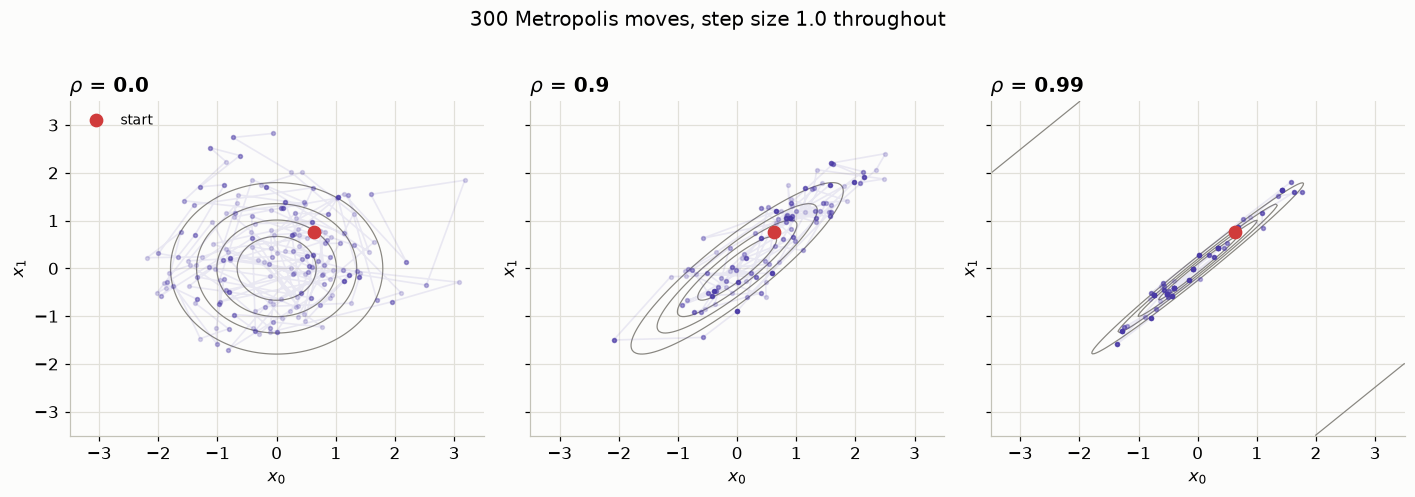
Read those left to right. At \(\rho = 0\) the chain wanders over the whole target; at \(\rho = 0.99\) it is pinned in a thin diagonal sliver, and the dark patches are where it sat still for many moves in a row. The proposal has not changed — only the shape it is trying to explore.
Now put a number on that.
def run_chains(log_target, step_size, n_chains=4, n_steps=25_000, warmup=5_000):
    """Several independent chains, so an ESS estimate is not one seed's luck."""
    kept, accs = [], []
    for c in range(n_chains):
        ch, a = metropolis(log_target, start=[0.0, 0.0], n_steps=n_steps,
                           step_size=step_size, seed=RANDOM_SEED + c)
        kept.append(ch[warmup:])
        accs.append(a)
    return np.stack(kept), float(np.mean(accs))     # (chain, draw, 2)


def ess_per_draw(chains):
    """Effective sample size, as a fraction of the draws taken.

    MCMC draws are **correlated**, so N of them carry less information than N
    independent ones. ESS answers "how many independent draws would this have
    been worth?" — so ESS/draw is near 1 for a sampler that is doing well, and
    near 0 for one that is barely moving. We read it off the first coordinate,
    which is all we need here.
    """
    dt = az.convert_to_datatree({"x": chains[..., 0]})
    return float(az.ess(dt, var_names=["x"]).x) / chains[..., 0].size


STEPS = [0.05, 0.1, 0.25, 0.5, 1.0, 2.0, 4.0]
sweep = []
for rho in RHOS:
    lt = log_target_gaussian(rho)
    for s in STEPS:
        chains, acc = run_chains(lt, s)
        sweep.append({"rho": rho, "step_size": s, "acceptance": acc,
                      "ESS/draw": ess_per_draw(chains)})
sweep = pd.DataFrame(sweep)
The squeeze
Sweep the step size at each correlation and look at what the best achievable ESS is.
fig, ax = plt.subplots(figsize=(7.0, 4.2))
for rho, colour in zip(RHOS, [S.ALT, S.PRIMARY, S.NAIVE]):
    block = sweep[sweep.rho == rho]
    ax.plot(block["step_size"], block["ESS/draw"], "o-", color=colour,
            label=f"$\\rho$ = {rho}")
ax.set(xscale="log", yscale="log", xlabel="step size", ylabel="ESS per draw",
       title="Every step size is bad once the target is a ridge")
ax.legend(fontsize=9)
fig.tight_layout()

best = sweep.groupby("rho")["ESS/draw"].max()
print("best ESS per draw, over all step sizes tried:")
for rho, v in best.items():
    print(f"  rho = {rho:<5} {v:.4f}"
          + ("" if rho == 0.0 else f"   ({best[0.0] / v:5.0f}x worse than rho = 0)"))
best ESS per draw, over all step sizes tried:
rho = 0.0 0.1273
rho = 0.9 0.0429 ( 3x worse than rho = 0)
rho = 0.99 0.0143 ( 9x worse than rho = 0)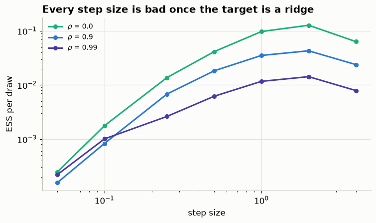
That is the difference from the mixture. There, tuning worked. Here every step size is bad, in one of two ways: small steps are almost always accepted but crawl, and large steps are big enough to travel the ridge but a circular step that large mostly lands off it sideways and is rejected.
There is no knife-edge setting you missed — the whole range is poor, and the best of it is far below what the same sampler manages on a round target.
⚠️ A correct-looking answer from a chain that did not work
The most dangerous cell in that table is the small-step one, because of what it reports about itself. Run it and look:
chains_bad, acc_bad = run_chains(log_target_gaussian(0.99), step_size=0.05)
n_draws = chains_bad[..., 0].size
ess_bad = ess_per_draw(chains_bad)

print(f"step_size 0.05, rho 0.99:  acceptance {acc_bad:.1%}")
print(f"  sd(x0) pooled over chains = {chains_bad[..., 0].std():.3f}"
      "   (the truth is exactly 1.000)")
print(f"  ESS/draw                  = {ess_bad:.5f}")
print(f"  -> about {ess_bad * n_draws:.0f} independent draws out of {n_draws:,}\n")

# The same quantity, chain by chain.
for c in range(chains_bad.shape[0]):
    x0 = chains_bad[c, :, 0]
    print(f"  chain {c}: mean x0 {x0.mean():+.2f}, sd {x0.std():.2f}"
          "   (true sd 1.00)")
step_size 0.05, rho 0.99: acceptance 84.4%
sd(x0) pooled over chains = 0.967 (the truth is exactly 1.000)
ESS/draw = 0.00022
-> about 17 independent draws out of 80,000
chain 0: mean x0 +0.50, sd 0.85 (true sd 1.00)
chain 1: mean x0 -0.04, sd 1.18 (true sd 1.00)
chain 2: mean x0 +0.43, sd 0.83 (true sd 1.00)
chain 3: mean x0 +0.13, sd 0.86 (true sd 1.00)A marginal standard deviation in the right neighbourhood is not evidence that the chain worked. This one lands within a few percent of the truth while containing a couple of dozen genuinely independent draws.
The per-chain numbers show the trick. Not one of the four gets the width right, and they do not even err in the same direction. Their means sit at different points, and that between-chain scatter refills roughly the variance the narrow chains are missing — so pooling manufactures a plausible number out of four separately wrong ones. That is the argument for running several chains and checking \(\hat{R}\), which is what notices the disagreement.
Which is the argument for doing both: pool several chains and check \(\hat{R}\), which is what notices that the chains disagree. Do not eyeball whether a summary looks plausible.
4. The same target, in PyMC
Two things are worth showing here. First, PyMC gives you Metropolis too, one argument away. It is not quite the sampler we wrote: for a vector-valued variable pm.Metropolis updates one coordinate at a time, with its own accept/reject for each — the coordinate-wise cousin of our blocked proposal. Hold that thought; section 5 is about what axis-aligned moves cost you. Second, and the reason this section exists: NUTS crosses this target without being tuned at all.
def gaussian_pymc_model(rho):
    """A PyMC model whose posterior IS the correlated Gaussian — no data needed."""
    cov = np.array([[1.0, rho], [rho, 1.0]])
    with pm.Model() as model:
        pm.MvNormal("x", mu=np.zeros(2), cov=cov, shape=2)
    return model


# `step=` picks the sampler. `pm.Metropolis()` must be constructed INSIDE the
# model context — outside it you get "TypeError: No model on context stack".
with gaussian_pymc_model(0.99):
    idata_mh = pm.sample(draws=2000, tune=2000, chains=2, cores=1,
                         step=pm.Metropolis(), progressbar=False,
                         random_seed=RANDOM_SEED)

print("Metropolis:")
print(az.summary(idata_mh, kind="diagnostics").to_string())
Sequential sampling (2 chains in 1 job)
Metropolis: [x]
Sampling 2 chains for 2_000 tune and 2_000 draw iterations (4_000 + 4_000 draws total) took 0 seconds.
We recommend running at least 4 chains for robust computation of convergence diagnostics
The rhat statistic is larger than 1.01 for some parameters. This indicates problems during sampling. See https://arxiv.org/abs/1903.08008 for details
The effective sample size per chain is smaller than 100 for some parameters. A higher number is needed for reliable rhat and ess computation. See https://arxiv.org/abs/1903.08008 for detailsMetropolis:
ess_bulk ess_tail r_hat mcse_mean mcse_sd
x[0] 8 7 1.24 0.34 0.28
x[1] 8 7 1.24 0.34 0.28ess_bulk in the single digits, and \(\hat{R}\) far past the 1.01 threshold — out of 4000 draws. PyMC prints warnings saying exactly this. Same model, same budget, NUTS:
with gaussian_pymc_model(0.99):
    idata_nuts = pm.sample(draws=2000, tune=2000, chains=2, cores=1,
                           nuts_sampler="pymc", progressbar=False,
                           random_seed=RANDOM_SEED)

print("NUTS:")
print(az.summary(idata_nuts, kind="diagnostics").to_string())
Initializing NUTS using jitter+adapt_diag...
Sequential sampling (2 chains in 1 job)
NUTS: [x]
Sampling 2 chains for 2_000 tune and 2_000 draw iterations (4_000 + 4_000 draws total) took 1 seconds.
We recommend running at least 4 chains for robust computation of convergence diagnosticsNUTS:
ess_bulk ess_tail r_hat mcse_mean mcse_sd
x[0] 703 868 1.00 0.037 0.026
x[1] 684 892 1.00 0.037 0.026The same two chains as paths, drawn exactly as before — so this is directly comparable to the hand-written sampler above and to Gibbs below. These are post-warmup draws, so both start somewhere sensible; the question is where they go from there.
N_SHOW_PYMC = 300
fig, axes = plt.subplots(1, 2, figsize=(11, 4.8), sharex=True, sharey=True)
for ax, (name, idt) in zip(axes, [("pm.Metropolis", idata_mh), ("NUTS", idata_nuts)]):
    path = idt.posterior.dataset["x"].values[0][:N_SHOW_PYMC]     # chain 0
    # A rejected proposal repeats the current point, so an "exactly repeated"
    # draw is a wasted iteration. NUTS has none: every draw is a new point.
    repeated = np.mean(np.all(np.diff(path, axis=0) == 0, axis=1))
    plot_path(ax, path, 0.99, f"{name}\n{repeated:.0%} of draws are repeats")
axes[0].legend(fontsize=9, loc="upper left")
fig.suptitle(f"{N_SHOW_PYMC} post-warmup draws at $\\rho = 0.99$", y=1.02)
fig.tight_layout()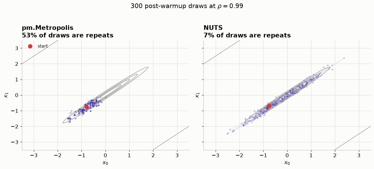
pm.Metropolis barely leaves the neighbourhood it started in, and over half its draws are exact repeats — rejected proposals, recorded again. NUTS repeats a small fraction of the time and otherwise lands somewhere new, far up or down the ridge rather than inching along it. In the same 300 draws it covers the whole target while Metropolis covers a corner of it.
That is what a gradient buys. NUTS follows the shape of the target instead of guessing at it, so the ridge stops being an obstacle and becomes a direction to travel in.
n_steps_mean = float(idata_nuts["sample_stats"].dataset["n_steps"].mean())
print(f"NUTS leapfrog steps per draw at rho = 0.99: {n_steps_mean:.1f}")
print("  (Metropolis has no analogue — it takes one cheap step and rejects it.)")
NUTS leapfrog steps per draw at rho = 0.99: 12.4
(Metropolis has no analogue — it takes one cheap step and rejects it.)It is not free, though: those long jumps cost many gradient evaluations per draw, and that count climbs as the geometry worsens.
That is the trade you want: ill-conditioning turns into a larger bill rather than into a confident wrong number. Metropolis, on the same target, stayed cheap and reported a posterior it had not actually explored.
5. Advanced: Gibbs has the same problem, for a different reason
(Skip if we are short on time — nothing later depends on it.)
You might reasonably suspect the trouble was our clumsy tuning. So take tuning off the table completely.
For this Gaussian the conditional distributions are known in closed form:
\[ x_0 \mid x_1 \;\sim\; \text{Normal}\!\left(\rho\, x_1,\ \sqrt{1-\rho^2}\right), \]
and symmetrically. A Gibbs sampler simply alternates: draw \(x_0\) given \(x_1\), then \(x_1\) given the new \(x_0\). There is no step size, no proposal and no rejection — every draw is exact and every draw is accepted.
def gibbs(rho, n_steps=25_000, seed=RANDOM_SEED, record_path=False):
    """Coordinate-wise Gibbs. Nothing to tune; acceptance is 1 by construction."""
    rng_g = np.random.default_rng(seed)
    sd = np.sqrt(1.0 - rho**2)
    x = np.zeros(2)
    chain = np.empty((n_steps, 2))
    path = [x.copy()]

    for i in range(n_steps):
        x[0] = rng_g.normal(rho * x[1], sd)      # x0 | x1
        if record_path:
            path.append(x.copy())
        x[1] = rng_g.normal(rho * x[0], sd)      # x1 | x0
        if record_path:
            path.append(x.copy())
        chain[i] = x

    return (chain, np.array(path)) if record_path else chain


gibbs_chains = {rho: np.stack([gibbs(rho, seed=RANDOM_SEED + c)[5_000:]
                               for c in range(4)])
                for rho in RHOS}

# For this target Gibbs turns each coordinate into an AR(1) process with lag-1
# correlation exactly rho^2 — so a sampler with NO knobs and a 100% acceptance
# rate is still provably slow here, by an amount you can write down in advance.
print(f"at rho = 0.99, Gibbs ESS/draw = "
      f"{ess_per_draw(gibbs_chains[0.99]):.4f}")
at rho = 0.99, Gibbs ESS/draw = 0.0111A sampler with no knobs, no rejections, and still two orders of magnitude short of independent draws.
The picture shows why:
# Same helper as the Metropolis paths above, so the two are directly comparable.
_, path_gibbs = gibbs(0.99, n_steps=100, seed=RANDOM_SEED, record_path=True)
path_mh, _ = metropolis(log_target_gaussian(0.99), start=[0.0, 0.0],
                        n_steps=100, step_size=1.0, seed=RANDOM_SEED)

fig, axes = plt.subplots(1, 2, figsize=(11, 4.8), sharex=True, sharey=True)
plot_path(axes[0], path_mh, 0.99, r"Metropolis, 100 moves")
plot_path(axes[1], path_gibbs, 0.99, r"Gibbs, 100 sweeps")
axes[0].legend(fontsize=9, loc="upper left")
fig.suptitle(r"Two samplers, the same ridge at $\rho = 0.99$", y=1.02)
fig.tight_layout()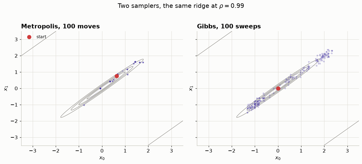
Every move is horizontal or vertical, because every move updates one coordinate. The ridge runs at 45°. So the chain can only climb it as a staircase of tiny right-angled steps, each limited by the width of the ridge rather than by its length. Nothing here is tunable: the constraint is the coordinate system, not the step length.
📝 Two very different algorithms, one ellipse
Gibbs has nothing to tune and rejects nothing, and it is still two orders of magnitude short of independent sampling along the ridge. That is what tells you the problem was never the algorithm.
One connection worth noticing: pm.Metropolis() from the previous section also updates a vector one coordinate at a time, so its moves are axis-aligned too and it inherits precisely this weakness.
6. When the problem is the posterior, not the sampler
Everything so far used a target we invented, with a correlation we chose. Now the cognitive model — where the same geometry shows up without anyone asking for it, and where you cannot fix it by changing sampler.
At 14:30 everything recovered cleanly. Here are two datasets from the same DDM, differing only in drift rate — and therefore in how often the participant makes an error.
from hssm.likelihoods import DDM
from ssms import Simulator

DRAWS, TUNE, CHAINS = 700, 700, 2
# z = 0.65 puts the start point above the midpoint, so the process begins nearer
# the "+1" boundary. That asymmetry is what makes the geometry legible later.
# v_balanced is set to land the error rate inside the 15-35% band that the
# design literature recommends — with a biased start point that takes a smaller
# drift than you might expect.
TRUE = {"v_balanced": 0.2, "v_extreme": 3.0, "a": 1.2, "z": 0.65, "t": 0.3}
PARAMS = ["v", "a", "z", "t"]


def make(v_true, n=600):
    o = Simulator(model="ddm").simulate(theta=[v_true, TRUE["a"], TRUE["z"], TRUE["t"]],
                                        n_samples=n, random_state=RANDOM_SEED)
    return np.column_stack([o["rts"].flatten(), o["choices"].flatten()])


def fit_ddm(observed, seed=RANDOM_SEED):
    with pm.Model():
        v = pm.Normal("v", 0.0, 3.0)
        a = pm.HalfNormal("a", 2.0)
        z = pm.Beta("z", 5.0, 5.0)
        t = pm.HalfNormal("t", 0.5)
        DDM("obs", v=v, a=a, z=z, t=t, observed=observed)
        # `initvals` is load-bearing, for the reason given in the 14:30 session:
        # PyMC would otherwise start `t` at 0.5, above the fastest RT in both of
        # these datasets (0.351 / 0.353). Beyond that point the DDM
        # log-likelihood is a flat constant, so a chain landing there has no
        # gradient to follow back and never recovers.
        return pm.sample(draws=DRAWS, tune=TUNE, chains=CHAINS, cores=1,
                         nuts_sampler="pymc", progressbar=False, random_seed=seed,
                         initvals={"t": np.array(0.1)})


fits, posteriors, error_rates = {}, {}, {}
for label, v_true in [("balanced", TRUE["v_balanced"]), ("extreme", TRUE["v_extreme"])]:
    obs = make(v_true)
    error_rates[label] = (obs[:, 1] == -1).mean()
    idata = fit_ddm(obs)
    fits[label] = idata
    p = idata.posterior.dataset
    posteriors[label] = {k: p[k].values.ravel() for k in PARAMS}
    print(f"{label:9s} error rate {error_rates[label]:5.1%}   "
          + "  ".join(f"{k}={posteriors[label][k].mean():5.2f}" for k in PARAMS))
print(f"\ntruth: v={TRUE['v_balanced']} or {TRUE['v_extreme']}, a={TRUE['a']}, "
      f"z={TRUE['z']}, t={TRUE['t']}")
Initializing NUTS using jitter+adapt_diag...
Sequential sampling (2 chains in 1 job)
NUTS: [v, a, z, t]
Sampling 2 chains for 700 tune and 700 draw iterations (1_400 + 1_400 draws total) took 4 seconds.
We recommend running at least 4 chains for robust computation of convergence diagnostics
Initializing NUTS using jitter+adapt_diag...balanced error rate 25.7% v= 0.22 a= 1.24 z= 0.63 t= 0.29Sequential sampling (2 chains in 1 job)
NUTS: [v, a, z, t]
Sampling 2 chains for 700 tune and 700 draw iterations (1_400 + 1_400 draws total) took 16 seconds.
We recommend running at least 4 chains for robust computation of convergence diagnosticsextreme error rate 0.0% v= 3.41 a= 1.42 z= 0.61 t= 0.28
truth: v=0.2 or 3.0, a=1.2, z=0.65, t=0.3The correlation structure is the diagnosis
fig, axes = plt.subplots(1, 2, figsize=(10, 4.2))
for ax, label in zip(axes, ["balanced", "extreme"]):
    d = posteriors[label]
    M = np.array([[np.corrcoef(d[i], d[j])[0, 1] for j in PARAMS] for i in PARAMS])
    im = ax.imshow(M, vmin=-1, vmax=1, cmap="RdBu_r")
    ax.set(xticks=range(4), yticks=range(4), title=label)
    ax.set_xticklabels(PARAMS); ax.set_yticklabels(PARAMS)
    for i in range(4):
        for j in range(4):
            ax.text(j, i, f"{M[i, j]:+.2f}", ha="center", va="center", fontsize=9,
                    color="white" if abs(M[i, j]) > 0.55 else S.TRUTH)
fig.colorbar(im, ax=axes, shrink=0.8, label="posterior correlation")
fig.suptitle("Every parameter pair, both designs", y=1.02)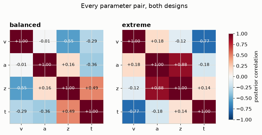
In the balanced design the correlations are moderate and structured. In the extreme design one pair dominates everything else: a with z, at +0.88.
The strongest pair in the extreme design is a with z — boundary separation against start point — and the weakest is v with a. That is worth pausing on, because v–a is the pair people reach for first.
For the extreme data a and z collapse together
With essentially no errors, every single trial ended at the same boundary. So ask what the data can possibly measure. The process starts at \(z\,a\) and has to travel
fig, axes = plt.subplots(1, 2, figsize=(10.5, 4.4))
for col, label in enumerate(["balanced", "extreme"]):
    d = posteriors[label]

    ax = axes[col]
    r = np.corrcoef(d["a"], d["z"])[0, 1]
    ax.plot(d["a"], d["z"], "o", color=S.PRIMARY, ms=2.5, alpha=0.25, ls="none",
            label="posterior draws")
    S.truth_point(ax, TRUE["a"], TRUE["z"])
    ax.set(title=f"{label}:  corr(a, z) = {r:+.2f}",
           xlabel="boundary separation $a$", ylabel="start point $z$")
    ax.legend(loc="lower right", fontsize=9)

fig.suptitle("The same ridge, in both designs", y=1.02)
fig.tight_layout()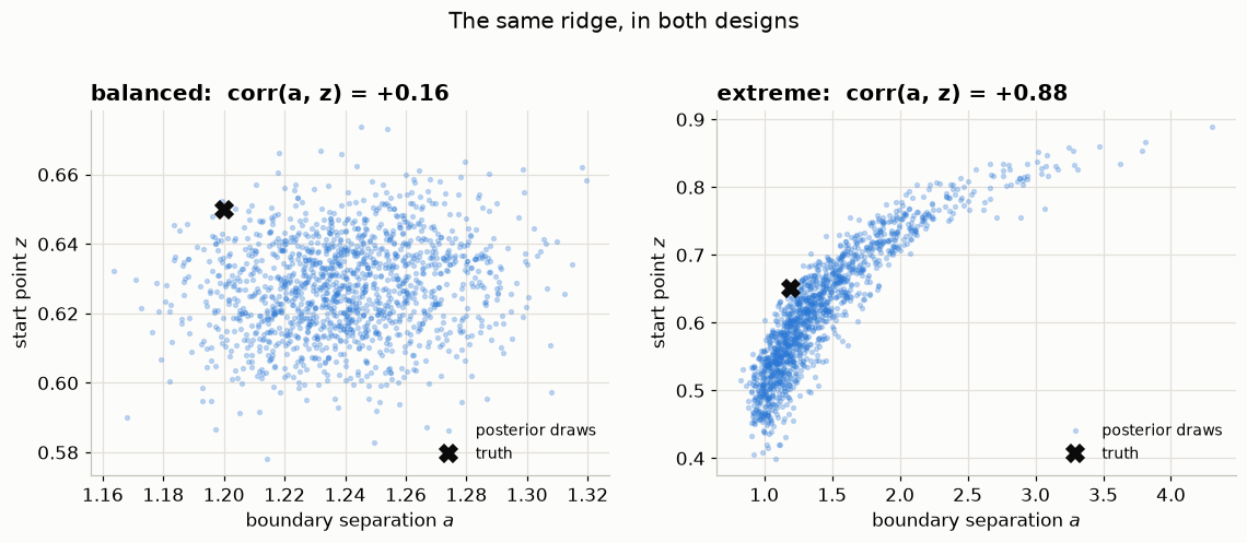
Left: a compact blob sitting on the truth. Right: a long thin ridge. The truth is on that ridge — but so is every other point along it, and the data have no way to say which.
All of it at once
a–z is the worst pair, but it is not the only one. The full pair plot shows every two-parameter view and the marginals down the diagonal — and the relationship between those two things is the point.
for label in ["balanced", "extreme"]:
    az.plot_pair(fits[label], var_names=PARAMS, marginal=True,
                 marginal_kind="kde")
    fig = plt.gcf()
    fig.set_size_inches(8.0, 8.0)
    fig.suptitle(f"{label} design — error rate {error_rates[label]:.1%}", y=1.01)
    fig.tight_layout()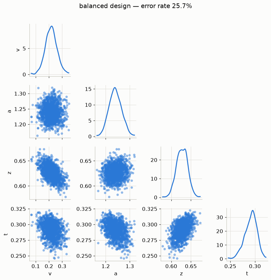
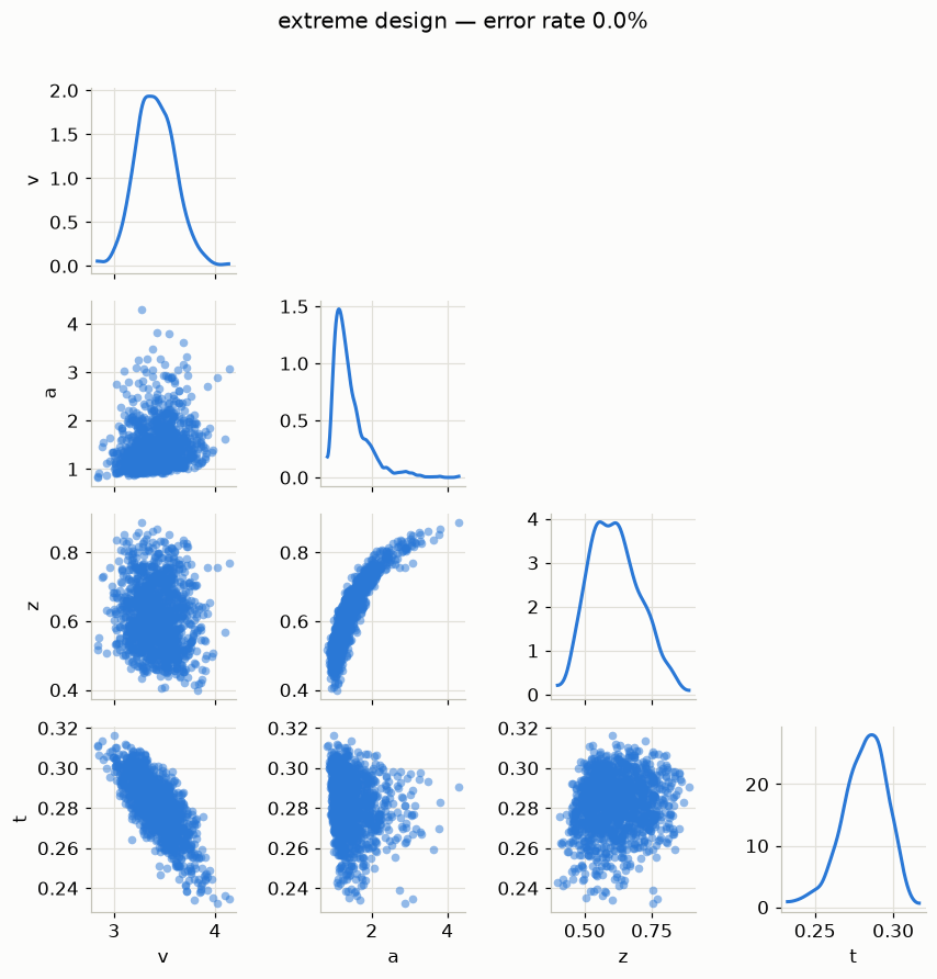
Poll. Look at the diagonal of the extreme-design plot — the marginal for each parameter on its own.
ahas a true value of 1.2, and its marginal smears from about 1 to beyond 4. Which conclusion follows?
- A. The data contain almost no information about
a.- B. The model is wrong.
- C. The data constrain
awell, but only jointly withz.- D. We need more trials.
Answer
C. The marginal for a is wide, but the joint is a thin ridge — meaning the data pin down a combination of a and z very precisely, and say almost nothing about where along that combination the truth sits.
A marginal is what you get after integrating out every other parameter. On a ridge, that integration sweeps along the entire ridge and returns something broad — which reads as “we learned nothing about a”, when what actually happened is “we learned a great deal about 2a(1-z) and nothing about the direction orthogonal to it.”
D is the tempting wrong answer, and yesterday’s reading settles it: more trials of the same design shrink both parameters’ marginals a little and leave the ridge exactly where it is. The ridge is a property of the design, not of the sample size.
🔑 Why this makes single-parameter conclusions hard
Most of what gets reported from a cognitive model is marginal: a posterior mean per parameter, a credible interval per parameter, a claim that boundary separation differs between groups. All of those read one axis of this picture at a time.
On a ridge that is a bad way to read it, in both directions:
- You will miss real effects. A wide marginal for
alooks like “no evidence”, so the interval comfortably includes zero difference and nothing gets reported. The information was there — it was in the joint, and marginalising threw it away. - You can manufacture false ones. Nudge anything that moves the ridge — a slightly different prior on
z, a different subset of trials — anda’s marginal slides along the ridge with it. The estimate moves a lot for reasons that have nothing to do with the effect you are testing.
What to do about it, in rough order of preference:
- Fix the design so the ridge does not form. Here that means an error rate that actually reaches both boundaries — the single most effective step, and the only one that adds information rather than redistributing it.
- Report the identified combination. If the data measure \(2a(1-z)\), say so and give an interval for that, rather than an uninterpretable interval for
a. - Compare models, not parameters. Fit with and without the effect and compare them; that question is often well-posed even when the individual parameter is not.
- Always look at the joint before reporting a marginal. Two minutes with
az.plot_pairis what stands between you and a confidently-worded claim about a parameter your experiment never measured.
What that costs you
fig, axes = plt.subplots(1, 4, figsize=(13, 3.4))
for ax, k in zip(axes, PARAMS):
    # Centre each design on ITS OWN truth, so the axis is estimation error and
    # the two designs are comparable even though true v differs between them.
    truth = {"v": None, "a": TRUE["a"], "z": TRUE["z"], "t": TRUE["t"]}[k]
    err = {lab: posteriors[lab][k] - (TRUE[f"v_{lab}"] if truth is None else truth)
           for lab in ["balanced", "extreme"]}

    lo = min(e.min() for e in err.values())
    hi = max(e.max() for e in err.values())
    bins = np.linspace(lo, hi, 60)

    ax.hist(err["extreme"], bins=bins, density=True, color=S.NAIVE, alpha=0.65,
            label=f"extreme ({error_rates['extreme']:.0%} errors)")
    ax.hist(err["balanced"], bins=bins, density=True, color=S.PRIMARY, alpha=0.85,
            label=f"balanced ({error_rates['balanced']:.0%} errors)")
    S.truth_line(ax, 0.0, axis="x")

    ratio = err["extreme"].std() / err["balanced"].std()
    ax.set(title=f"${k}$ — {ratio:.1f}x wider", xlabel=f"estimate $-$ true ${k}$",
           yticks=[])
axes[0].set_ylabel("density")
axes[0].legend(fontsize=8, loc="upper left")
fig.suptitle("Same model, same number of trials — only the error rate differs",
             y=1.03)
fig.tight_layout()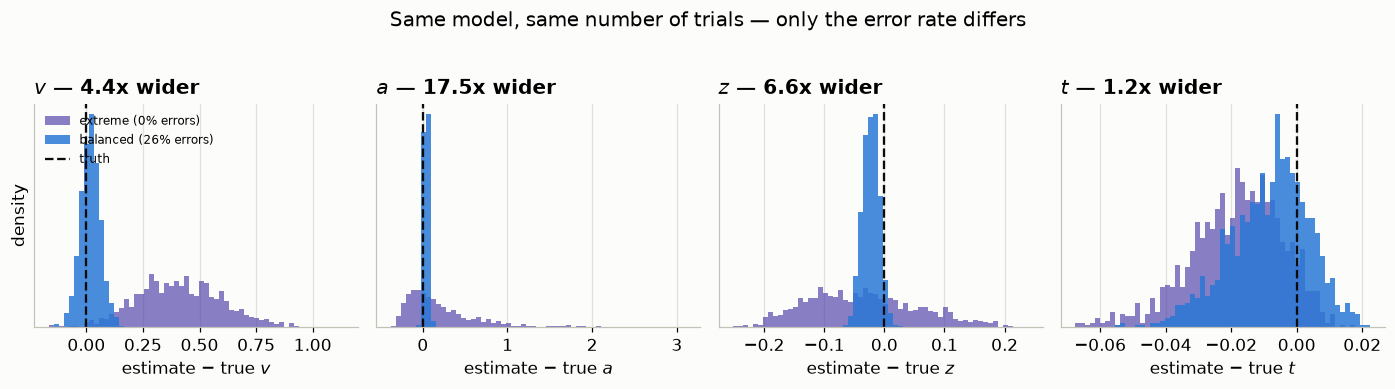
🔑 High accuracy is bad data for parameter estimation
This is the counterintuitive headline, and the damage is targeted rather than uniform. Read the panel titles: a blows up by an order of magnitude and z several-fold, while t is essentially untouched. Those are exactly the parameters that a design where one boundary is never reached cannot see. Nothing is wrong with the sampler and nothing is wrong with the model — the experiment did not collect the information.
Notice that t is barely affected while a blows up. The damage is not spread evenly.
Whether the point estimates also come out biased varies from dataset to dataset, which is itself worth noticing: on a ridge, where the posterior mean lands depends on where the prior and the little remaining information happen to pull it. Sometimes you get lucky. You cannot tell from one fit which case you are in — that is the problem.
Exercise
We set the true start point to z = 0.65, above the midpoint. Predict what happens to corr(a, z) if you push it to 0.80, then check.
Answer
Change TRUE["z"] and re-run the extreme-design fit. The a–z correlation stays strong — it is around +0.84 to +0.90 anywhere in this range, because the mechanism does not depend on which boundary wins, only on the fact that one of them always does.
What does change is a itself: the distance travelled is \(a(1-z)\), so a larger z means a smaller a reproduces the same data, and the posterior for a shifts down accordingly.
The instructive part is what happens if you go the other way and set z = 0.5 with a balanced drift. Both trade-offs weaken at once, because now both boundaries get reached and the data can see both distances. Identifiability is a property of the design, not of the model.
Next, tomorrow at 11:00: today’s difficulties came from correlation that is roughly the same everywhere in parameter space. Hierarchical models bring a nastier relative — curvature that changes as you move — where the failure stops being inefficiency and becomes bias.